Decision making

Download the slides here

Introduction¶

This week’s sections don’t cover a single theme. Instead, we’ll look at a few different strands of work in neuroscience that could be of interest to people with a machine learning or quantitative background. We may also add more sections in future years.

In this section, we’ll focus on decision making - a really broad topic of course, because in a way you can think of everything the brain has to do is about making decisions.

Two-alternative forced choice (2AFC)¶

Let’s make this even more concrete with a very specific sort of task, the two-alternative forced choice, or 2AFC.

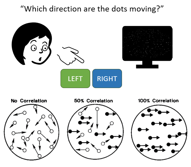
In this task, participants are shown some sort of image or movie and asked to decide between two options. A common one is the random dot kinematogram, with random dots on the screen some of which are moving coherently either to the left or right, and some moving randomly. The participants have to determine which direction the coherent dots are moving, and sometimes they’re asked to make their decision as quickly as possible. The reaction time is the time between the start of the video and the moment when they press the button.

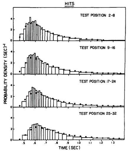
If you run this experiment, you see characteristic skewed distributions of reaction times. This data is actually from a slightly different task where participants were asked whether or not they had seen the image being shown before or not.

Drift diffusion / random walk model¶

There’s a beautifully simple theory for how we make these decisions which can account for these reaction times:

• Imagine that as time goes by, sometimes a bit of evidence arrives that is on its own unreliable, but suggestive that the dots are moving right rather than left. Then another, followed by one that suggests that left is more likely, and so on. We keep track of a running total of how much evidence we’ve received that suggests right versus left, and once it crosses some threshold we make our decision. This is a biased random walk, where it’s more likely we take a step in the correct direction than the wrong direction.

• As we increase the number of time points from 10 to 30.

• Then from 30 to 100.

And all the way up to 1000, this random walk looks more and more like Brownian motion with a drift. This gives us a mathematical theory that lets us analytically compute expressions for the reaction time distributions.

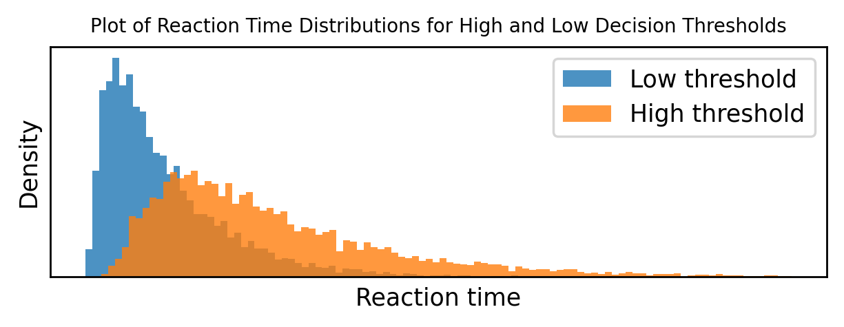
• Or we can just numerically plot them, here with either a low decision threshold or a high decision threshold.

• And sure enough, we get something that looks very much like the data from experiments.

Probabilistic interpretation¶

That’s nice, but still this model might seem a bit ad hoc. Fortunately, it turns out that there’s a neat probabilistic interpretation of this model.

• Let’s set up a probabilistic model of the task. We’ll say there’s a true direction $D$ that can be either $L$ or $R$, and both options are equally likely. You can actually modify this to make the options have different probabilities too.

• Now we have the data observed at time t is a series of symbols $𝑋_𝑡$ each of which is $R$ or $L$.

• The probability you observe the correct symbol is $p$ and the probability you observe the incorrect symbol $1-p$.

• Now given we know the observed data and we want to infer the unknown value of $D$, we compute which of the two options is more likely. We’ll write that as $\textcolor{#a503fc}{r(X)}$ equals the ratio of the probability that $D=R$ given the observations $X$, divided by the probability that $D=L$. If this ratio is high then $D=R$ is much more likely, and if it’s low then $D=L$ is more likely.

• We use Bayes’ theorem to rewrite the probability that $D=R$ given X in terms of the probability of $X$ given $D=R$ times the probability $D=R$ over the probability of $X$. And the same thing for the probability that $D=L$ on the bottom.

• The $\textcolor{#128f04}{P(X)}$ cancels and both the prior probabilities $D=R$ and $D=L$ are both ½ so they cancel too.

• The observations at different time points are independent, so we can expand these as a product of the probabilities at each time point.

• And this product is the same at the top and bottom so we can pull it out.

• Now to see what’s going on more clearly we take the log of this ratio to get the log likelihood ratio.

• The log of a product is the sum of the logs.

• And we’ll write the individual terms as the “evidence at time $t$” $\epsilon(𝑋_𝑡)$.

• This evidence will be log of $\textcolor{#03bafc}{𝑝}/ 1- \textcolor{#03bafc}{𝑝}$ when $𝑋_𝑡=𝐿$. If $𝑋_𝑡=𝑅$ it’s log of $(1- \textcolor{#03bafc}{𝑝})/ \textcolor{#03bafc}{𝑝}$ but this is just negative log of $\textcolor{#03bafc}{𝑝} / 1- \textcolor{#03bafc}{𝑝}$.

• With that we can write the log likelihood ratio as a constant term multiplied by the sum of terms $\textcolor{#fc0505}{\Sigma_{t}\delta(𝑋_𝑡)}$ which are +1 if $𝑋_𝑡=𝑅$ and -1 if $𝑋_𝑡=𝐿$.

• But this sum is precisely the random walk we saw previously.

• When D=R the sum increases by 1 with probability $\textcolor{#03bafc}{𝑝}$ and decreases by 1 with probability $1-\textcolor{#03bafc}{𝑝}$, and vice versa if $D=L$.

• We can understand the decision threshold in terms of probability now. We wait until the log likelihood ratio is bigger than some threshold θ or equivalently that the likelihood ratio is bigger than $𝑒^{\theta}$.

• And this happens when the sum of the deltas is bigger than some threshold, precisely as in the drift diffusion model.

Electrophysiological data¶

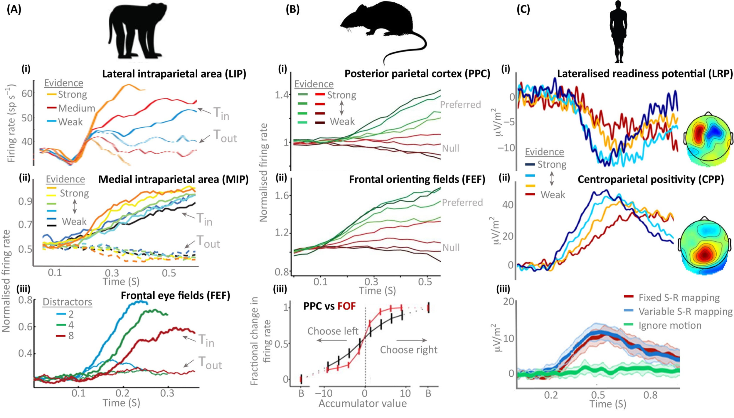
And finally, perhaps the best thing about this theory is that having come up with the model based on fitting behavioural observations and then finding a rigorous probabilistic interpretation, electrophysiological experiments find traces of these evidence accumulation processes across multiple different brain regions in multiple species.

Of course, it’s never quite as clean cut as the theory and all sorts of modifications have been proposed, like adaptive thresholds that get closer to the origin over time to represent the increasing urgency of making some sort of decision, or thresholds that adapt to wider context in various ways. There are also much more comprehensive Bayesian theories of decision making in which this model is just one special case, and so on.