Introduction
In the last section we learnt about how we can acquire neural data.
Data
Regardless of what method we use to collect our data we’re going to end up with a matrix like this where:
- One axis is time.
- The other is neurons.
- Each cell denotes the activity of one neuron at one time point. Activity here could be binary - in the case of spikes, or continuous in the case of calcium imaging data or spikes binned into spike rates (i.e., number of spikes per time window).

Figure 1:Neural data can be represented as a matrix of neurons x time, where each cell denotes the activity of neuron i at time t.
One thing to note is that rather than recording neural activity continuously, experimentalists will often conduct multiple trials with a fixed length. So time may be discontinuous. For example, an experiment could be composed of trials where a subject is shown images which they’re asked to classify, with breaks in-between.
With this sort of data there are lots of different questions we could ask like:
- How do different neurons behave?
- Are there neurons which are only active on some trials or on some part of a trial?
- Does this change over trials? For example, maybe as the animal learns the task (or gets bored).
- If we have some information about where the neurons are in the brain, then we can see if neurons with different response properties are located in different spatial locations.
- If we were working with data from an artificial neural network, an equivalent approach could be comparing the units in different layers.
Once we have a question or questions in mind we can then decide on an appropriate analysis method.
Analysis methods
There are lots of different approaches to analyzing neural data, so I’m just going to highlight three. A simple approach is to calculate summary statistics.
For example, in a classification task we could compute how strongly each neuron responds to each class, and then see how specific it’s response is. Or if we were varying a stimulus parameter continuously, like the brightness of a screen, we could see how tuned to this parameter each neuron is (i.e., how activity changes as a function of this parameter).
So what does this analysis look like?
Summary statistics
In Fyhn et al. (2007) the authors let a rat freely move around a square area while recording the activity of neurons in part of the brain known as the hippocampus.
In the left panel, the black line shows the animal’s path, and the red dots show the locations in space where one neuron spiked. Then the right panel, shows a heatmap of the neuron’s firing rate, with red being high. So, this heatmap is equivalent to a 2d tuning curve, and we can see that this neuron is tuned to a specific location in this environment.
Neurons with responses like these are known as place cells, they were first discovered in 1971 O’Keefe & Dostrovsky, 1971, but are still an active area of research.
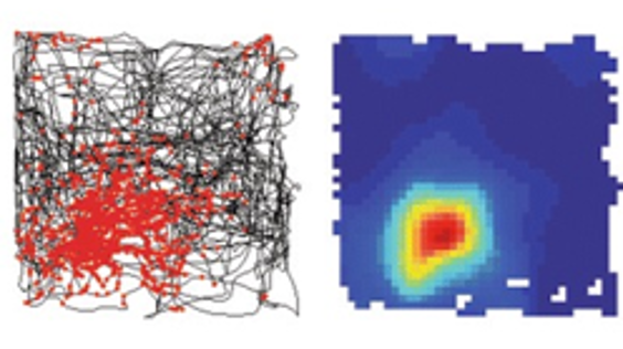
Figure 2:Place cells spike at specific locations within an environment Fyhn et al., 2007.
However, many neuron’s aren’t so clearly tuned to specific environmental features and rather than thinking of single neurons as encoding variables it may be better to try to understand what information populations of neurons encode.
This brings us onto our second approach which is neural decoding.
Neural decoding
The aim of neural decoding is to use neural activity to estimate something about the environment or subject. For example, if we think about the rat, we could take its neural activity and try to estimate its velocity or position in the environment. To do that we could start from our matrix (of neurons by time), bin the spikes into bins to get continuous firing rates - which are easier to work with, and then use data from multiple bins to predict our variable of interest at a specific time.
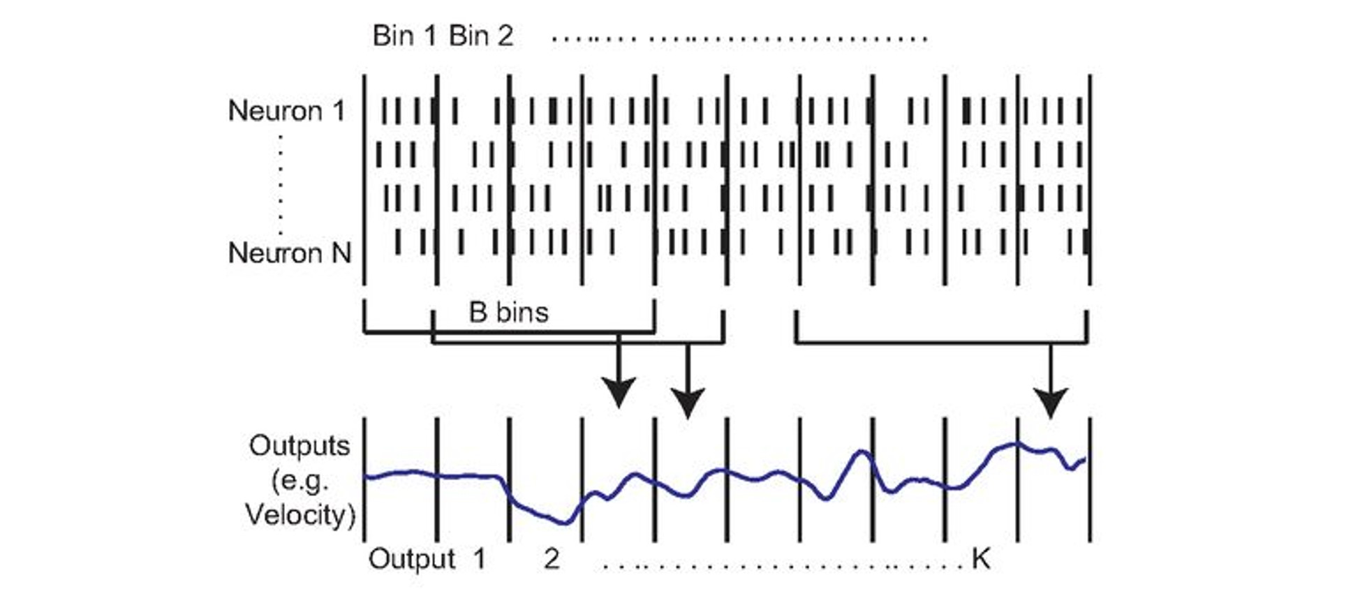
Decoding attempts to relate neural activity to other variables. For example, the animal’s velocity Glaser et al., 2020.
As this is essentially a regression problem, there are many approaches we could use to do this like using filters or neural networks, and Glaser et al. (2020) compares these methods in detail. For example, in this image, each point on the x-axis represents a different decoding approach, and then the y-axis shows how accurately each method can decode the rat’s location and you can see that some methods can do this quite accurately, even though the dataset only has 50 neurons.
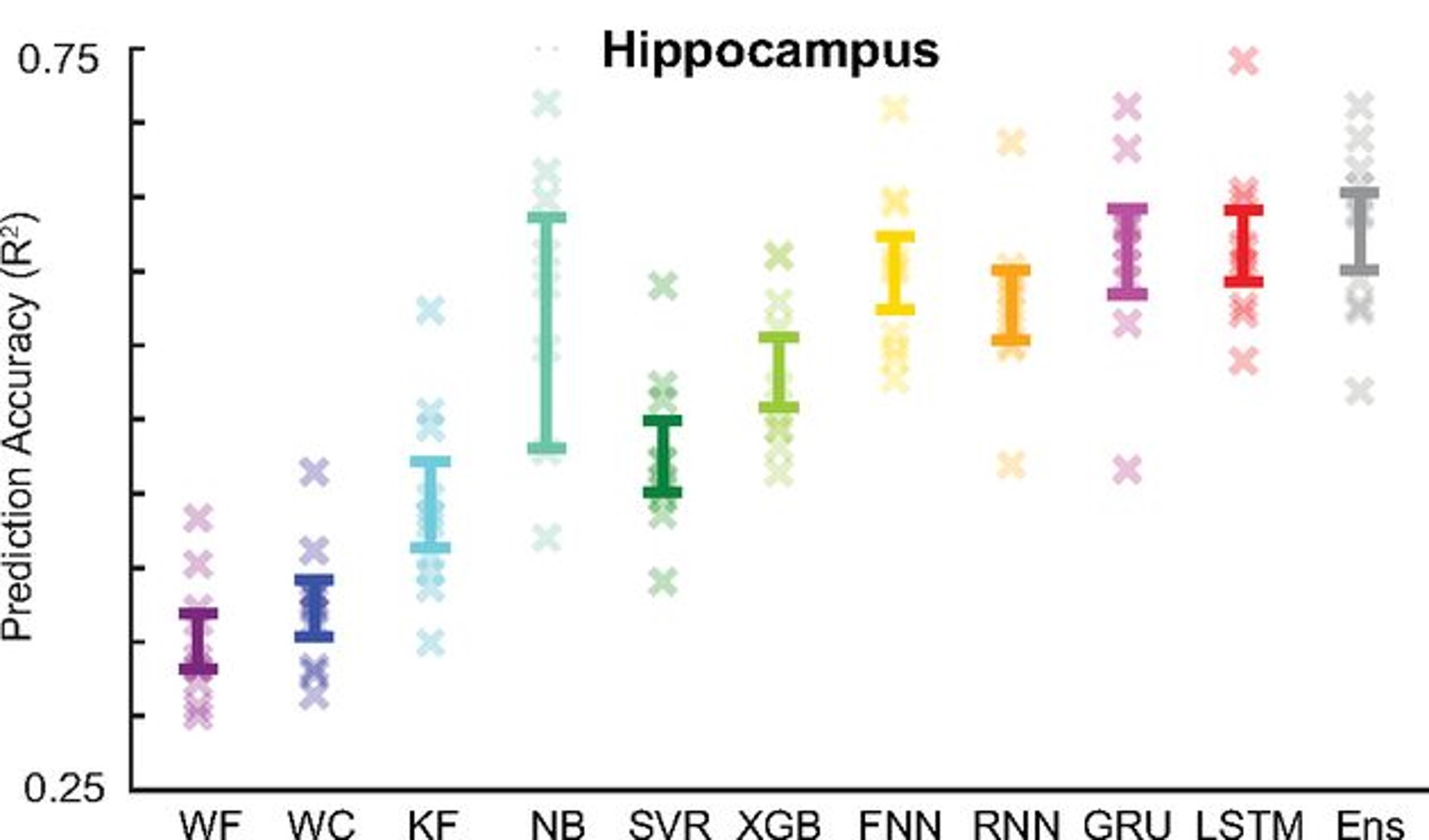
Figure 4:Decoding accuracy (y-axis) across a range of different decording approaches (x-axis) Glaser et al., 2020.
But if we tried to decode location from another population of neurons somewhere else in the brain, like visual cortex, our results would be much worse, and so we can use decoding accuracy to estimate what information is present in different brain areas. However, decoding relies on having a variable or variables of interest to estimate, and sometimes we may not have that: for example, if we’re just recording spontaneous brain activity.
In that case, one approach would be what we’re going to call ensemble methods.
Neural ensembles
These methods try to identify groups of neurons with correlated patterns of activity over time (which we term ensembles).
One approach to this would be to use a clustering algorithm to group the neurons into clusters with similar activity patterns. Another is the method shown here, which is called tensor component analysis.
Here, we take our 2d matrix of neurons recorded over time and trials, and reshape it to a 3d tensor of neurons by time by trials, then describe this tensor using a set of ensembles - each of which is described by three vectors (shown in red, green and blue).
- A neuron factor - which notes how strongly associated each neuron is with that ensemble.
- A temporal factor - which notes how that ensembles activity changes over the course of a trial.
- A trial factor - which shows how the activity of the ensemble changes over trials.
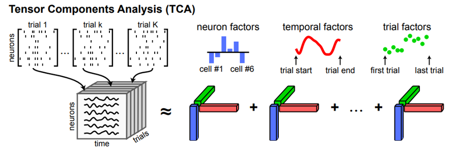
Figure 5:Tensor component analysis Williams et al., 2018.
This may seem a bit abstract, so let’s see what it yields when applied to real data.
This experiment is still focussed on spatial navigation but we’ve switched to mice, and what we call a plus maze - which you can see in panel A. Essentially the mouse starts in either the east or west arm, has to navigate to either the north or the south, and then if it’s correct it receives a reward.
So, what does applying tensor component analysis to the neural data recorded during this experiment reveal?
Here each row shows one of 8 ensembles, and then each column shows that ensembles neuron, temporal and across-trial factors. Working through these:
- In the neuron factors column - the x-axis shows all of the 280 recorded neurons, and then each y-axis shows how strongly associated each neuron is with each factor. So, you can see that different neurons are associated with different ensembles.
- In the temporal factors column - the x-axis shows time across each trial, and each y-axis shows the activity of each ensemble. So, you can see that different ensembles are active at different times during the trial.
- Finally, in the across trials column each dot shows a single trial, the x-axis shows the order of the trials, and then each y-axis shows how active each ensemble was on a given trial. And the dots are coloured by the different trial properties shown in B.
For example - if we focus on ensemble 2:
- It’s temporal factor shows us that these neurons are mostly active at the start of a trial, and
- It’s trial factor shows that these neurons are more active on trials when the mouse starts in the east than the west arm of the maze (compare the yellow and purple dots).
Now try to interpret the other ensembles yourself.
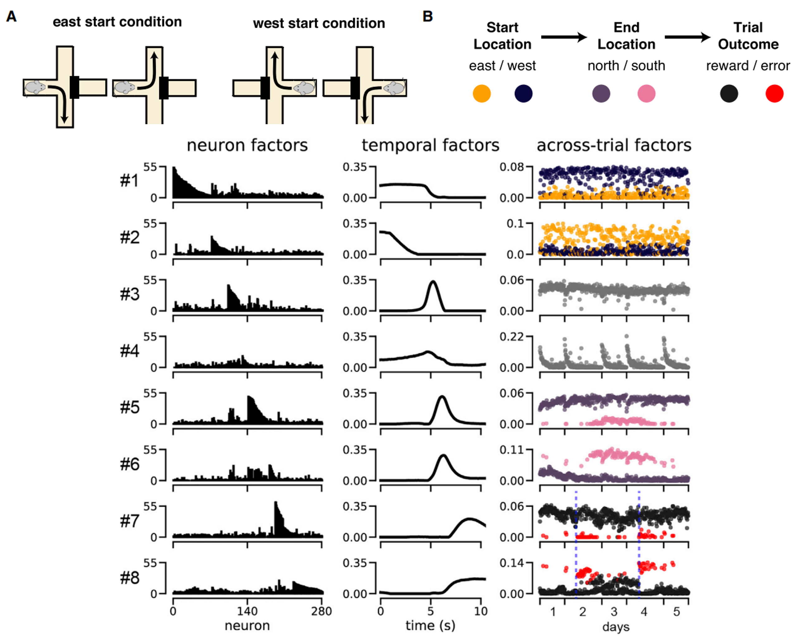
Figure 6:Tensor component analysis applied to a mouse navigation experiment Williams et al., 2018.
Summary
Hopefully, this section has taught you a bit about how we can analyse neural activity data using summary statistics, decoding methods and ensemble methods. But there are many other methods too, so we would encourage you to read around.
- Fyhn, M., Hafting, T., Treves, A., Moser, M.-B., & Moser, E. I. (2007). Hippocampal remapping and grid realignment in entorhinal cortex. Nature, 446(7132), 190–194. 10.1038/nature05601
- O’Keefe, J., & Dostrovsky, J. (1971). The hippocampus as a spatial map. Preliminary evidence from unit activity in the freely-moving rat. Brain Research, 34(1), 171–175. 10.1016/0006-8993(71)90358-1
- Glaser, J. I., Benjamin, A. S., Chowdhury, R. H., Perich, M. G., Miller, L. E., & Kording, K. P. (2020). Machine Learning for Neural Decoding. Eneuro, 7(4), ENEURO.0506-19.2020. 10.1523/eneuro.0506-19.2020
- Williams, A. H., Kim, T. H., Wang, F., Vyas, S., Ryu, S. I., Shenoy, K. V., Schnitzer, M., Kolda, T. G., & Ganguli, S. (2018). Unsupervised Discovery of Demixed, Low-Dimensional Neural Dynamics across Multiple Timescales through Tensor Component Analysis. Neuron, 98(6), 1099-1115.e8. 10.1016/j.neuron.2018.05.015