Introduction
Neuroscience, machine learning and computing more generally have had a long and rich history of influencing each other. There’s no way we can cover everything that could be said about that, so in this section we want to just pick out a few threads in that history, and show how the influence goes both ways.
The neural network
Let’s start by talking about the idea of the neural network.
One of the first papers to mathematically model this was from McCulloch & Pitts (1943). This ultimately led to the modern study of neural networks in both biology and machine learning.
Their approach was to take what was known at that time about the biology of neurons, explicitly acknowledge what they still didn’t know, and create an abstract model that would work even with future findings.
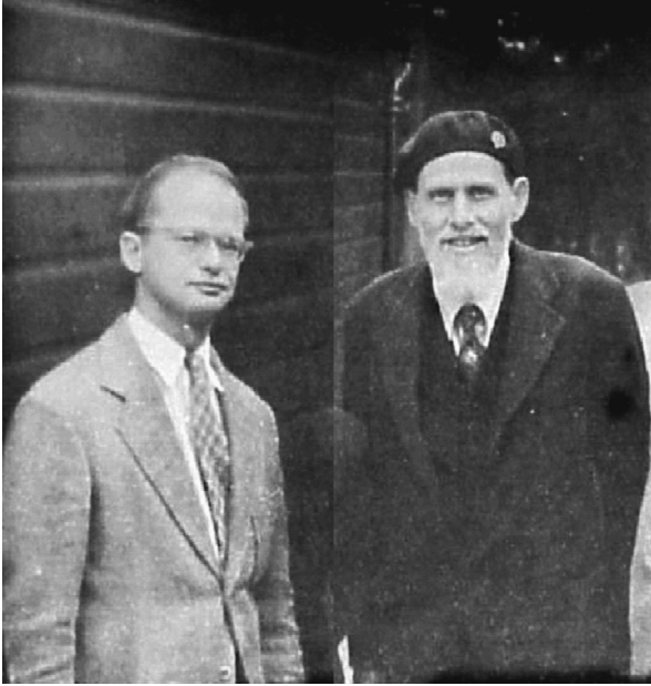
Figure 1:McCulloch and Pitts (1949). From Moreno-Díaz & Moreno-Díaz (2007).
This model is essentially equivalent to the modern artificial neuron, except that input and output activations are binary and weights are plus or minus 1. This matched what was known at the time that biological neurons communicate via discrete all-or-nothing bursts of activity called action potentials or spikes, that we’ll come back to next week.

Figure 2:McCulloch and Pitts’ neuron model.
Even today, this is not a terrible model of networks of neurons, although it misses out on a lot of interesting temporal dynamics that we’ll talk about throughout the course.
The main result they showed was that the class of functions computable by these networks was equivalent to propositional logic. In other words, you could implement any logical function with neural networks, and vice versa.
The next major development in the neural network concept was from Frank Rosenblatt who invented the perceptron model that is still used in a modified form today Rosenblatt, 1958.
And yes, he actually built it with wires because they didn’t have computers that could simulate them at that time. It had 512 modifiable connections and filled an entire room, using motors to modify the weights.
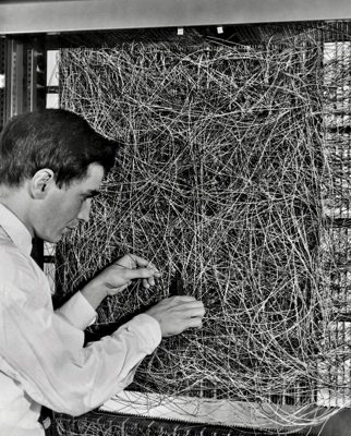
Rosenblatt’s insight was that the McCulloch and Pitts model and its close links with propositional logic was too rigid to handle the statistical problems the brain has to contend with. Namely, that biological networks seem to be wired up at least partly randomly, they are very noisy and so is the input data from the world they are handling.
The model he came up with is actually fairly complicated and we won’t go into it in detail. Like McCulloch and Pitts it uses binary activations and had a recurrent structure and temporal dynamics inspired by what was known from biology at the time.
Later work simplified it to the form you have probably seen before.
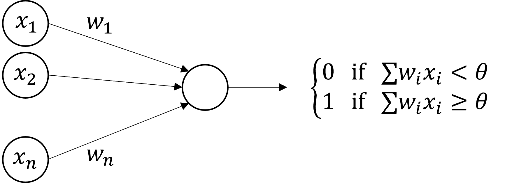
Figure 5:Modern formulation of Rosenblatt’s perceptron.
The key result of this work was to show that given enough training data from a distribution, the test accuracy on different samples from the same distribution approaches the training accuracy, something that wasn’t true of the earlier approaches and definitely an important property for understanding the brain.
The next development we have to talk about is Minsky’s criticisms of the perceptron Minsky & Papert, 2017. We won’t say much about this since it doesn’t bear directly on neuroscience, but it feels wrong not to mention it at all.
During the 1960s Marvin Minsky started criticising the perceptron ultimately leading to a book in 1969 that is credited with ending funding for neural network research and setting back the field for decades.
We’re not going to take a position on that, but there are a couple of interesting things to say about his criticisms in terms of the history we’re talking about.
His argument was that a single layer perceptron could only implement a linearly separable function, and therefore couldn’t compute functions like:
- Exclusive-OR
- Evenness
- Connectedness
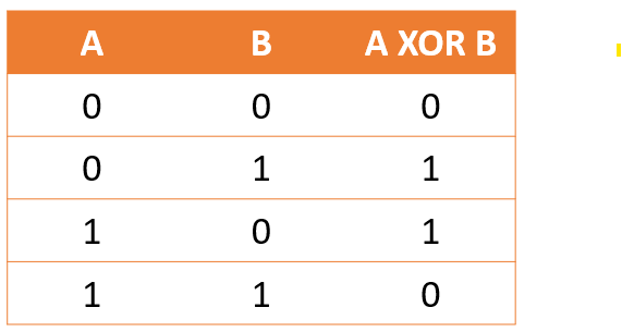
(a)XOR problem.
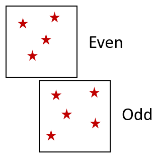
(b)Even-odd problem.

(c)Connectedness problem.
Figure 6:Some of Minsky’s challenges for single layer perceptrons.
However, he did recognise that multilayer perceptrons were able to do so, and indeed it was well known that the McCulloch and Pitts networks could do exclusive-OR for example, because it could do any logical function.
His criticism of multilayer perceptrons was not that they couldn’t implement these functions, but that they were too hard to train. Obviously, that turned out to be largely wrong, which we’ll come back to in a moment. But it is interesting to note that it wasn’t entirely wrong.
Although it’s possible to solve the connectedness problem with a deep or recurrent neural network, it’s still very hard to find this or any other solution via training, without essentially feeding in the answer in terms of a very specific and highly constrained architecture.
It’s still an open research question, and to justify talking about this in a history of neuroscience and ML, the latest paper we could find on the topic was actually from a neuroscience research group Larsen & Druckmann, 2022.
Backpropagation
Minsky thought that multilayer neural networks would be hard to train, but Rumelhart et al. (1986) found a solution in backpropagation.
We’re going to assume you either already know what backpropagation is, or will be learning about it in another course very soon. The box below has a summary. In brief, they found an efficient algorithm to compute the gradient of the loss function with respect to the parameters of the network, and therefore an efficient way to do gradient descent on multilayer neural networks.
Mathematical background on backpropagation
Want to minimise scalar loss with a vector of parameters θ.
Compute the gradient
The gradient .
The vector chain rule applies to a pair of composed functions:
Define the Jacobian matrix .
Then the chain rule says .
So we can efficiently compute the gradient just by matrix and vector multiplications.
Gradient descent
- Choose a learning rate α.
- Update parameters according to the rule .
- Note that much better algorithms exist!
This has proven to mostly solve Minsky’s problem with trainability, including finding a solution to the XOR problem. Although it is still not theoretically proven when it should work, and we saw a moment ago an example where it fails.
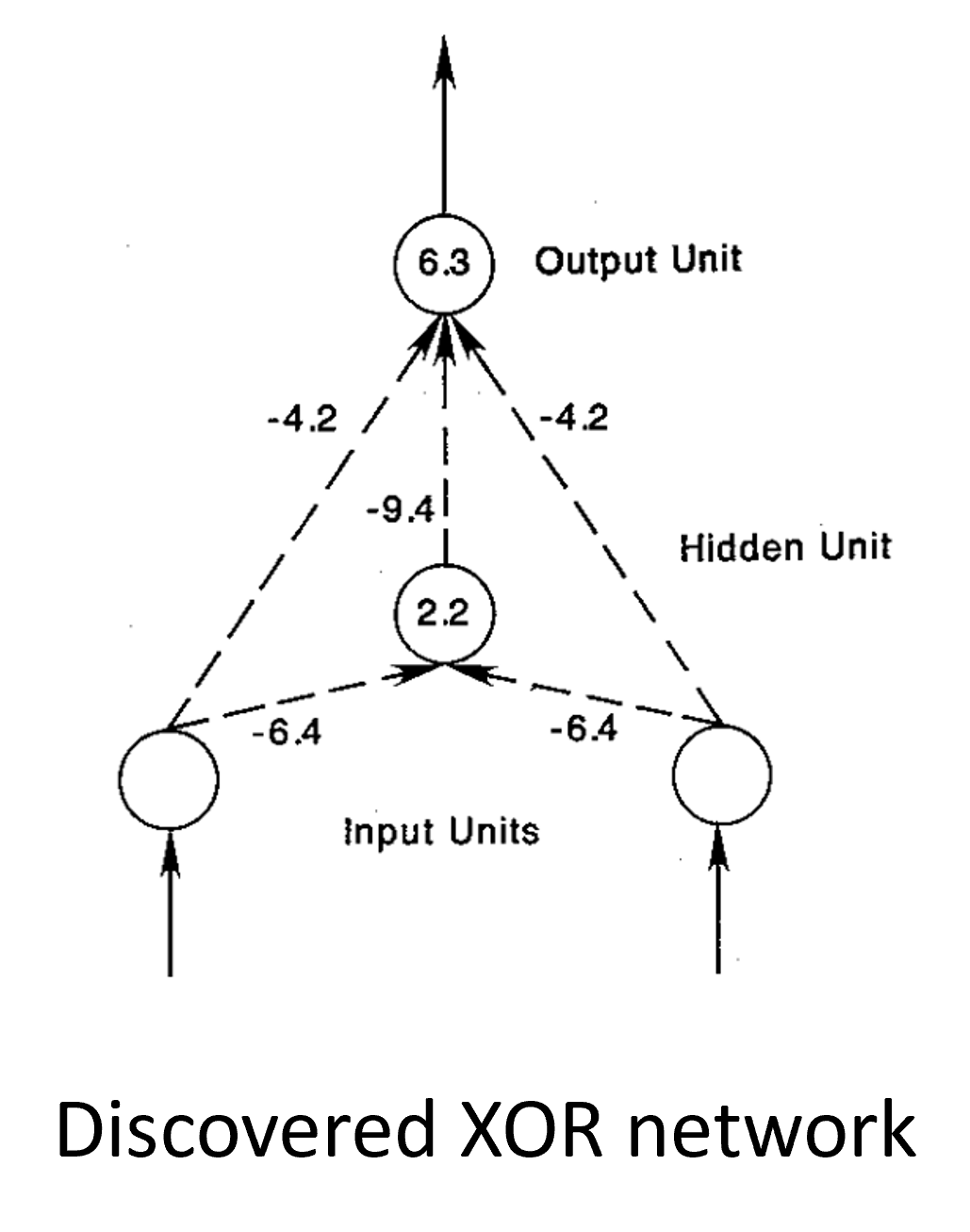
Figure 7:Solution to Minsky’s XOR Problem
Incidentally, gradient based methods were known in the 60s when Minsky was developing his arguments, but they were considered to be too inefficient and slowly convergent for high dimensional problems.
Returning to neuroscience, Rumelhart and colleagues explicitly recognised that although their method was effective, it wasn’t biologically plausible. But there are some interesting twists to this:
- The first is that some biologically plausible learning rules can be seen as mathematical approximations of backprop, which we’ll talk about later in the course.
- The second is that the reason that backprop isn’t biologically plausible may turn out to be irrelevant.
The argument goes that backprop requires passing an error signal backwards through the network, and there’s no biological mechanism that can do that.
You could do it with a secondary feedback network that carries the error signal backwards through the network, but it would have to be exactly symmetrical with the feedforward network, and nothing like that has been observed in the brain.
But in a fascinating development from 2016 onwards, Timothy Lillicrap and colleagues found that if you just use a random feedback network that isn’t symmetrical, it still works Lillicrap et al., 2016Lillicrap et al., 2020!
It turns out that the feedforward network learns to align itself with the feedback network so that in the end the feedback network is carrying the correct error signals for the learned - or aligned - feedforward network.
This ‘feedback alignment’ turns out not to scale to very deep networks, but the story isn’t over yet and there’s still a lot of interesting research going on in this space.
The visual system and convolutional neural networks
OK, so we’re done with talking about neural networks in general and want to cover just a couple more topics before finishing this section.
The first is the interplay between neuroscientific studies of the visual system, and the development of the convolutional neural network.
In the late 50s and early 60s, neuroscientists Hubel and Wiesel discovered two types of cells dominated in the early part of the visual system Hubel & Wiesel, 1959Hubel & Wiesel, 1962.
Most of the cells they analysed had a receptive field, that is a small, local area of the visual field where shining light could cause the neuron to fire, and in the rest of the field it has no effect. This is roughly equivalent to saying that they act as linear filters.
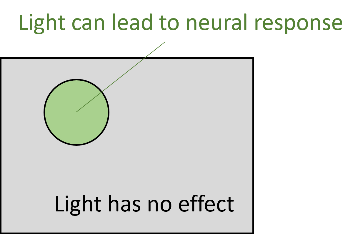
Figure 8:Receptive field.
Here you can see one example from their recordings.
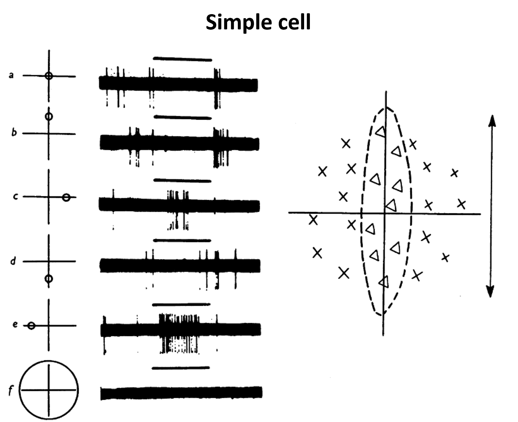
Figure 9:Simple cell recorded by Hubel and Wiesel.
Shining a light where the x’s are caused the cell to be more active, and shining it where the triangles are caused it to be less active.
They also found complex cells. These were defined to be any cell that wasn’t simple, but in many cases they found that they had the property of responding to a bar of light with a preferred orientation, but they didn’t mind where in their receptive field the bar was shown.
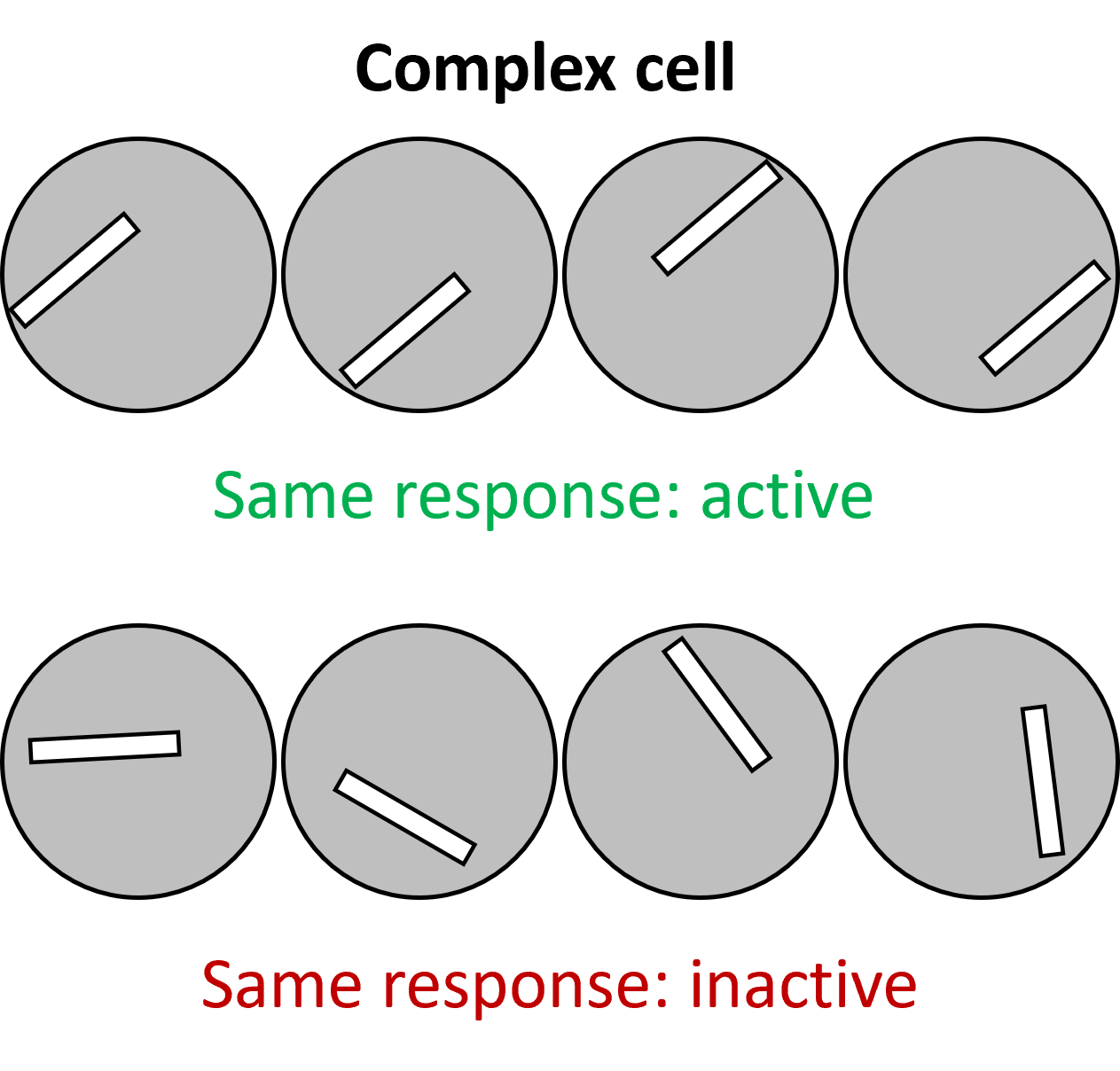
Figure 10:Complex cell response.
If you know about how convolutional neural networks work, this result probably doesn’t surprise you. You can think of simple and complex cells as convolutional layers and pooling layers.
The simple and complex cell structure was the direct inspiration for Fukushima’s 1980 “Neocognitron” Fukushima, 1980. This was an explicit computational model inspired by Hubel and Wiesel, and featured alternating S and C-layers, corresponding to simple and complex cells. The network was trained by a bespoke unsupervised learning rule that we won’t go into here.

Figure 11:Neocognitron architecture, from Fukushima (1980)
In 1989 Yann LeCun and others took essentially the same architecture but trained it using backpropagation, later refining this model and calling it a convolutional neural network LeCun et al., 1989Lecun et al., 1998.
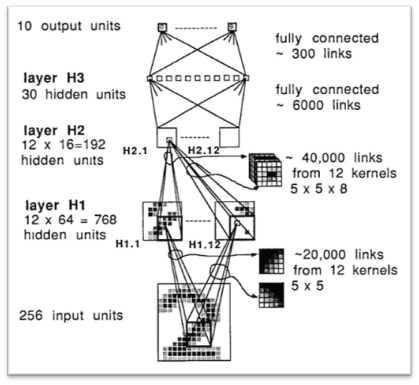
(a)1989 convolutional neural network.
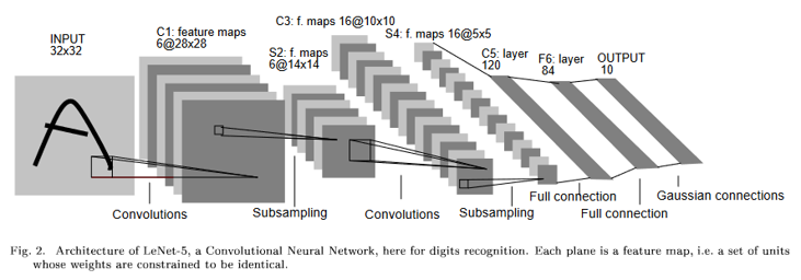
(b)1998 convolutional neural network.
Figure 12:Evolution of LeCun’s convolutional neural network.
This led to a flurry of work in machine learning over the next decades and played a big part in the current explosion of success in machine learning.
Before closing out this discussion of the visual system, we want to briefly take it back to neuroscience and show that the influence isn’t just one way.
Yamins et al. (2014) found that training a CNN to perform well at a task actually gave internal representations that were a close match to neural data recorded in the visual system. Kell et al. (2018) found the same thing in the auditory cortex. This led Schrimpf et al. (2018) to propose a “brain score” and leaderboard to track which models gave the closest match to neural data.
But the story isn’t over, and there are lots of people out there who are not convinced by this:
- Jacob et al. (2021) found that these networks don’t predict the patterns of success and failure made by humans on out-of-distribution stimuli.
- Weerts et al. (2021) found the same problem in auditory stimuli, and Adolfi et al. (2023) found the same thing independently around the same time.
So, the jury is still out on how good deep neural networks are as models of the brain, but one thing for sure is that machine learning is having an outsized influence on neuroscience at the moment.
Reinforcement learning
The last thing we’re going to talk about in this video is reinforcement learning. The phrase actually dates back to Pavlov in 1927 - yes the dog guy. The study of this sort of learning though actually goes back to Thorndike (1898).
At this point it wasn’t neuroscience so much as animal psychology. He built cages with opening mechanisms of varying complexity that the animals had to escape from, and tracked how long it took for them to escape over repeated trials. You’ll find these look remarkably like modern day training curves.
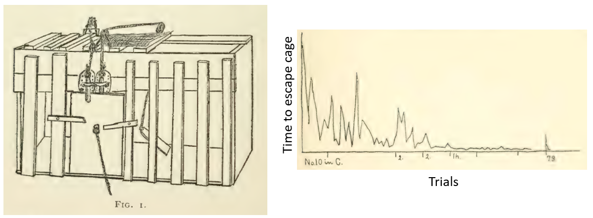
Figure 13:Reinforcement learning experimental setup from Thorndike (1898).
In his conclusion, you can even see some hints of what in modern reinforcement learning terms we’d call optimising for value instead of optimising for reward.
our view abolishes and declares that the progress is not from little and simple to big and complicated, but from direct connections to indirect connections in which a stock of isolated elements plays a part, is from ‘pure experience’ or undifferentiated feelings, to discrimination, on the one hand, to generalizations, abstractions, on the other
There’s a lot of developments in this space from researchers in psychology and neuroscience, and we won’t go into the whole history of this topic. If you’re interested in it, there’s a great book from Sutton and Barto that is freely available online and goes deep into the history.
Here we’ll just mention a few interesting moments from that history:
Like Alan Turing’s 1948 paper where he describes a computational learner that is explicitly described as a model of cortex Turing, 2004.
When a configuration is reached for which the action is undetermined, a random choice for the missing data is made and the appropriate entry is made in the description, tentatively, and is applied. When a pain stimulus occurs all tentative entries are cancelled, and when a pleasure stimulus occurs they are all made permanent.
There’s then a long spell where the mathematical modelling of reinforcement learning is primarily carried out by computer scientists and people working in optimal control (Bellman 1950s, Minsky 1950s-60s, Klopf 1980s, Watkins 1989 Q-learning).
It came back to neuroscience in a big way in the 80s and 90s with experiments on dopamine neurons, and models that showed that their activity corresponded to what you’d expect from temporal difference learning (Schultz).
This sparked a huge wave of work in neuroscience, a lot of which was going at the Gatsby Computational Neuroscience unit at UCL led by Peter Dayan and colleagues (e.g. Montague et al. (1996)).
And just to show that there’s a tight relationship to this day, Demis Hassabis’ last academic post before founding DeepMind in 2010 was at UCL with Peter Dayan in 2009. And he’s still advocating for AI to be influenced by neuroscience Hassabis et al., 2017.
What next?
This has been a very brief and incomplete history of some of the ways that neuroscience and machine learning have interacted over the years. There’s a lot more!
- McCulloch, W. S., & Pitts, W. (1943). A logical calculus of the ideas immanent in nervous activity. The Bulletin of Mathematical Biophysics, 5(4), 115–133. 10.1007/bf02478259
- Moreno-Díaz, R., & Moreno-Díaz, A. (2007). On the legacy of W.S. McCulloch. Biosystems, 88(3), 185–190. 10.1016/j.biosystems.2006.08.010
- Von Neumann, J. (1945). First draft of a report on the EDVAC. Moore School of Electrical Engineering, University of Pennsylvania. 10.5479/sil.538961.39088011475779
- Rosenblatt, F. (1958). The perceptron: A probabilistic model for information storage and organization in the brain. Psychological Review, 65(6), 386–408. 10.1037/h0042519
- Goodman, D. F., Benichoux, V., & Brette, R. (2013). Decoding neural responses to temporal cues for sound localization. eLife, 2. 10.7554/elife.01312