Rate-based models

Download the slides here

General form¶

In this section we’ll only discuss learning of a synaptic weight $\color{#0f73bf}{w}$, in response to a pre-synaptic neuron firing spikes at a rate $\color{#b35f10}{r_\pre}$, and a post-synaptic neuron firing at a rate $\color{#b80909}{r_\post}$.

We model this with a differential equation saying that the weight changes at a rate $\color{purple}{\tau_w}$ proportionate to some function $F$ of the weight and the pre- and post-synaptic weights.

Different functions $F$ give you different models.

Simplest possible Hebbian rule¶

That’s quite abstract, so let’s take a look at a concrete example.

Let’s choose the function $F$ to be the product of the pre- and post-synaptic firing rates so that $w$ just grows in proportion to the correlation between the firing rates.

This clearly satisfies the idea of “Cells that fire together ($\textcolor{#b35f10}{r_\pre}$ and $\textcolor{#b80909}{r_\post}$ both large) wire together ($\textcolor{#0f73bf}{w}$ grows)”

But we can already see a problem with this. There’s no reason for the weight to stop growing ($\textcolor{#0f73bf}{w}$ grows without bound). It will keep just getting bigger and bigger. This actually turns out to be an issue with a lot of learning rules, and we’ll keep coming back to it.

One solution is to have a hard bound, just clip w at some maximum value:

Another solution is a softer bound which just reduces the rate of change of the weight as you get close to the maximum value. There are various ways you can do this, this equation is just one example:

Another problem is that in this simple formulation, the weight will only grow, never get smaller, since both the pre- and post-synaptic firing rates are always positive. It is possible to fix this by adding another term, but let’s move on to another model.

Oja’s learning rule¶

Oja’s learning rule was designed to solve the problem of the weights growing without bound. You take the standard Hebbian rule and subtract off a term proportionate to the product of the weight and the square of the postsynaptic firing rate. In other words, after growing for a while the weights will stop changing.

This has two nice properties:

• The first is that as hoped for, the weights don’t keep growing.
• The second is more surprising: this learning rule extracts the first principal component of its inputs. A link between a biological learning rule and a statistical or machine learning algorithm: principal component analysis.

We’re going to see how to prove this, and it gets a bit hairy. So to keep things a simpler, we’ll make a couple of assumptions that are not quite right. We’ll look at the case of a vector of inputs $\bold{x}$ and a single linear output neuron $y$. So we can write $y$ as the dot product of the weight and the inputs.

We’ll assume the vector $\bold{x}$ represents the pre-synaptic firing rates, but we’re also going to assume it has mean value 0.

This won’t change the result but makes the analysis simpler. With these assumptions, we can rewrite the learning rules like this, using a dot above the $\bold{w}$ to indicate a derivative, and replacing 1 over time constant with γ.

Oja’s learning rule analysis¶

Now let’s get into the hairy mathematical analysis. You might want to work through this on a piece of paper. We start with the same setup up as before, with a vector of inputs $\mathbf{x}$ and a single output $y=\mathbf{w}^\intercal\mathbf{x}$.

The rate of change of the weight follows this equation:

and the output $y$ follows this equation:

Note that since $y$ is a scalar, the dot product of weight $\bold{w}$ and input $\bold{x}$, we can write as $\bold{w}^\intercal \bold{x}$ or $\bold{x}^\intercal \bold{w}$.

We’re interested in the fixed point after a long period of time when no more learning is happening. In other words, when on average the rate of change of $\bold{w}$ is 0. We’re using the angle brackets to mean an average.

Expanding out $\mathbf{\dot{w}}$, we get this:

Replacing $y$ with either $\bold{w}^\intercal \bold{x}$ or $\bold{x}^\intercal \bold{w}$ you get this - you’ll see why we did it like this in a moment.

Note that the mean of $\bold{x} \mathbf{x}^\intercal$ is $\bold{C}=\langle \mathbf{x}\mathbf{x}^\intercal\rangle$, the covariance matrix of $\bold{x}$. Using this, we can rewrite the equation above like this.

Since $\bold{w}^\intercal \bold{Cw}$ is a scalar, which we’ll call λ, this equation becomes:

But this means that λ is an eigenvalue of $\bold{C}$ and $\bold{w}$ is an eigenvector. This is exactly the definition of $\bold{w}$ being a principal component. In fact, you can show that Oja’s rule will always converge to the first principal component, but that analysis is more complicated. Because we get this fixed point of $\bold{w}$, we know that $\bold{w}$ doesn’t grow without bounds, and we can actually show a bit more than that by computing the fixed point of the norm of $\bold{w}$, defined as:

We set its derivative to 0 and expand:

Expanding the derivative out using the formula we calculated above, we get:

This is satisfied when $|\mathbf{w}|^2=1$. In other words, we get weight normalisation from Oja’s rule.

BCM rule¶

We’ve seen that Oja’s rule keeps weights bounded and leads to the neuron learning principal components. Another approach is the BCM rule, named after Bienenstock, Cooper and Munro Bienenstock et al., 1982. Their aim was a model of the development of selectivity in the visual cortex, and so they set out to find a learning rule that maximises selectivity. They defined this as 1 minus the mean response of the network divided by the maximum. In other words, for high selectivity, overall, the network should respond very little, but for certain inputs it should have a very strong response.

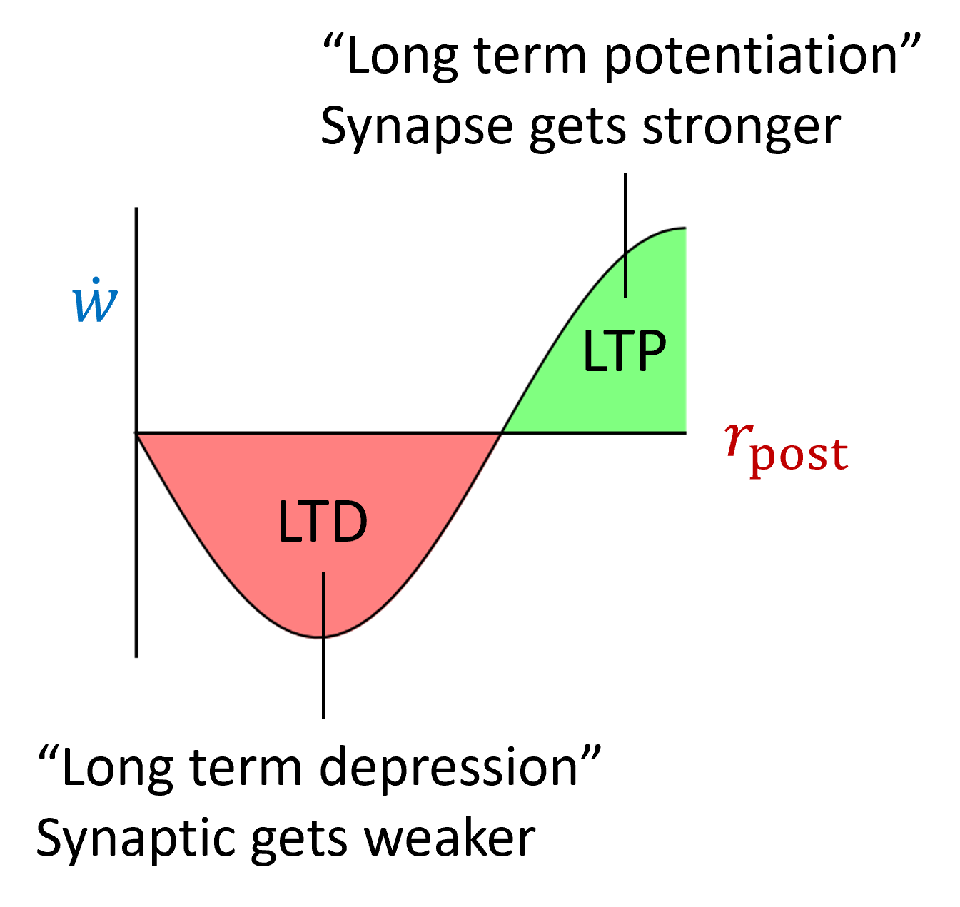
Their rule multiplies the simple Hebbian rule from before with a term that can be positive or negative. It’s positive if the postsynaptic firing rate is high, and negative if it’s low. High and low and controlled by a threshold $\textcolor{#18a326}{\theta}$.

This means that synapses can get stronger or weaker. The intuition here is that it promotes selectivity because those inputs that cause a high firing rate will be driven even higher, and those with a low firing rate even lower. However, you can already see that if $\textcolor{#18a326}{\theta}$ is just a constant, there’s nothing to stop this from blowing up. Once the post-synaptic firing rate goes above $\textcolor{#18a326}{\theta}$ it can just keep growing without bounds.

So they made $\textcolor{#18a326}{\theta}$ into a dynamic variable that averages the square of the postsynaptic firing rate. If you imagine a learning environment where different inputs are constantly being presented, you can imagine this either as a running average over time, or as a running average over the whole dataset.

Now if $\textcolor{#b80909}{r_\post}$ gets too large, the threshold will increase and the sign changes to negative and the synapse will weaken. Similarly, if $\textcolor{#b80909}{r_\post}$ gets too small it will strengthen it. So the output rate shouldn’t go to 0 or ∞

It also encourages selectivity because if $\textcolor{#b80909}{r_\post}$ is equal to $\textcolor{#18a326}{\theta}$ as it would be if all inputs led to the same output, then you’d be at this fixed point. However, this fixed point is unstable as a slight perturbation would push you away from the fixed point. Hence this rule is making sure you don’t settle in a fixed point where the selectivity is low.

You can imagine that at the start of learning, the output firing rate is low for all inputs, but higher for some than others. The threshold will lower until one of the inputs gives a rate above the threshold. At that point, the weights that respond to this input will get stronger. This increase in the firing rate will cause the threshold to increase, and so the weights corresponding to all the other inputs will decrease, and the network will end up selective to just that one preferred input.

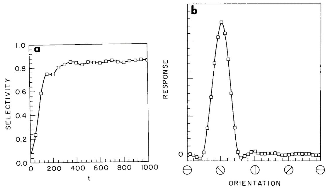
Sure enough, you can see that happening in their model of orientation selectivity in the visual cortex. Over time, the selectivity increases, and the end result is a network with a strong preference for one particular orientation. This qualitatively matches what happens in development.

Incidentally, you might wonder why do we take the square of the firing rate. Well, the exact choice of taking the square isn’t essential. It’s only important that it be nonlinear for reasons we won’t go in to here.

Summary¶

We’ve seen how Hebb’s principle can be translated into learning models based on firing rates, and that this can generate quite interesting computational properties like doing principal component analysis or developing feature selectivity. However, it misses an important feature which is the timing of spikes. We’ll turn to that in the next section.