STDP

Download the slides here

Introduction¶

Spike Timing-Dependent Plasticity (STDP) is a form of Hebbian learning that takes the timing of individual spikes into account.

Experimental measurement¶

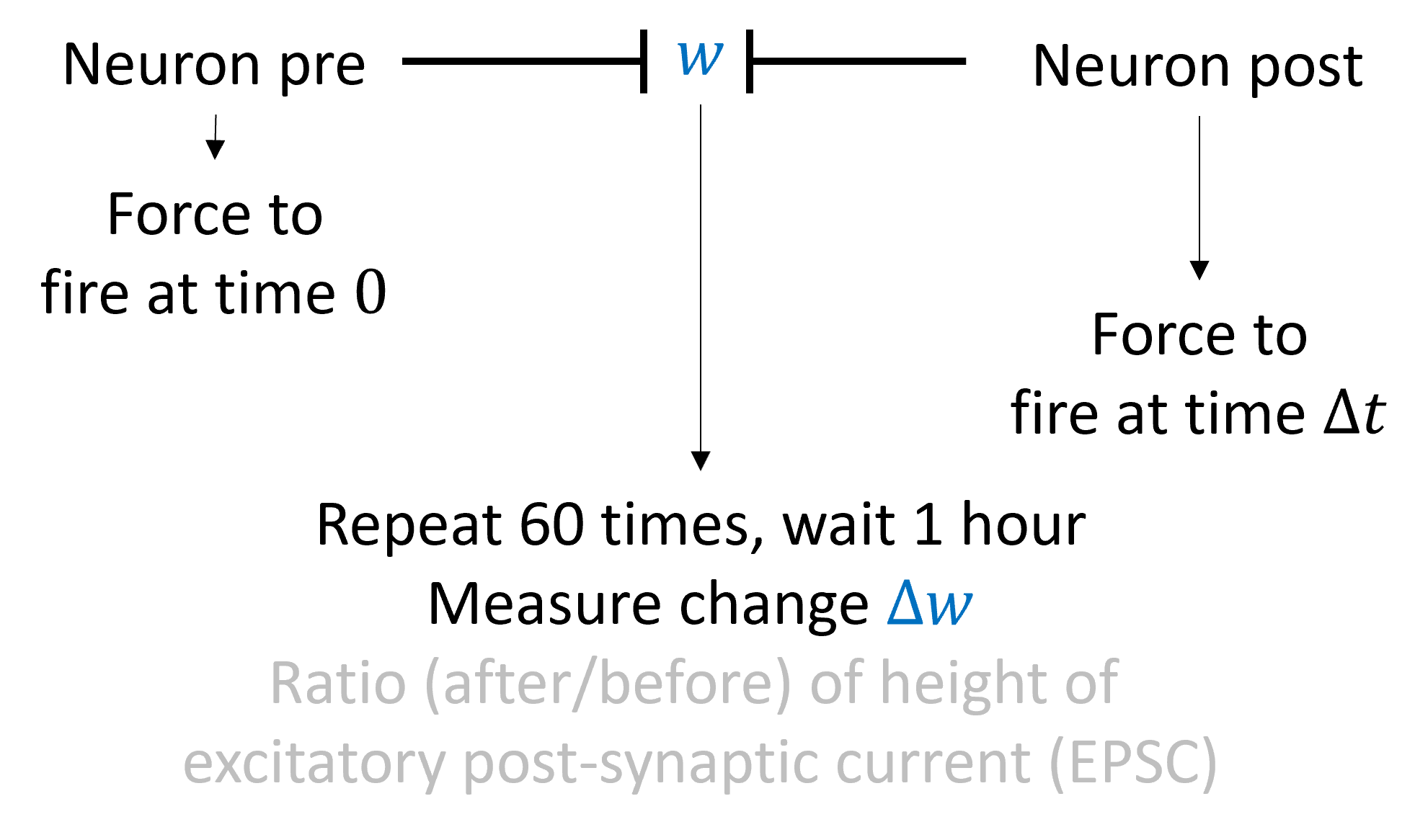
Let’s start with how it’s measured. We find a pair of neurons connected by a synapse. We then force the pre-synaptic neuron to fire a spike at time 0 and the post-synaptic neuron to fire a spike at time $\Delta t$. We then repeat this pairing about 60 times, wait around an hour, and measure the change in the synapse. We measure this by computing the height of a post-synaptic current from a single excitatory spike before and after the pairing.

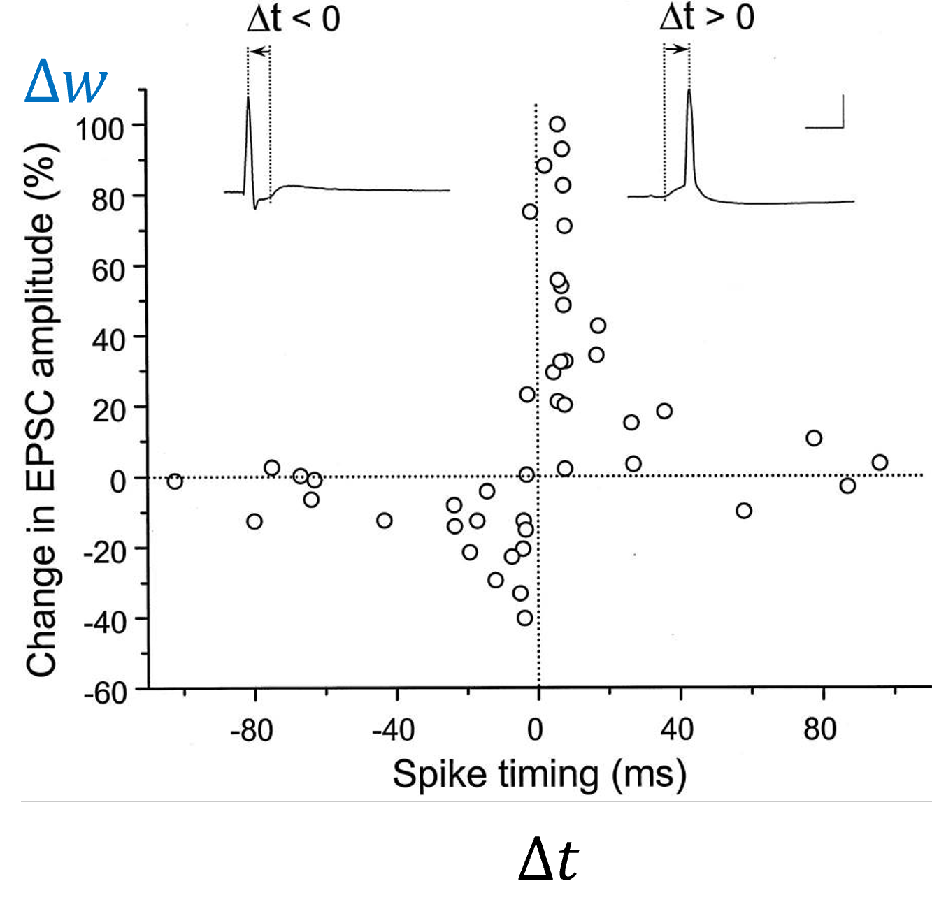
And we get results that look like this. It’s a bit noisy, but you can generally see that if the post-synaptic neuron fires after the pre-synaptic neuron, the weight goes up. If the post-synaptic neuron fires before the pre-synaptic neuron, the weight goes down. The closer in time, the stronger the effect.

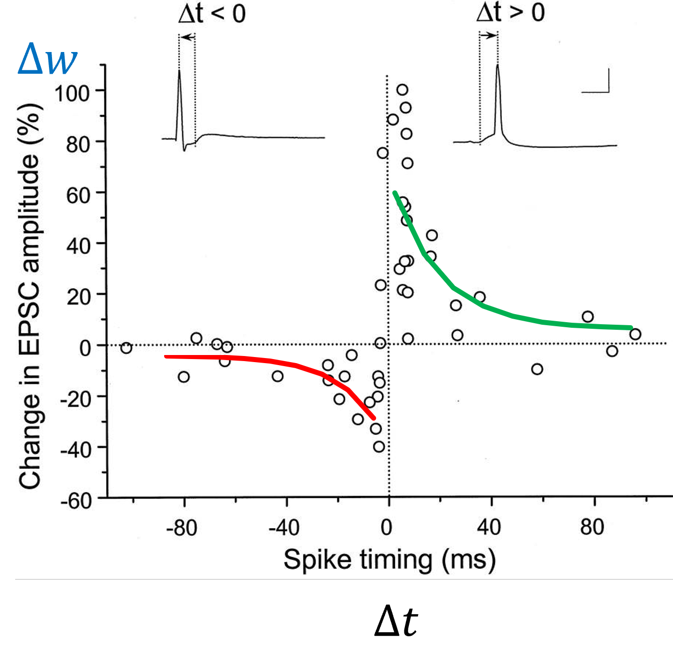
We can roughly fit this with a pair of exponentials with different heights and time constants:

Shown in this figure:

We talked before about Hebbian learning (what fires together, wires together) but this is actually closer to what Hebb originally suggested. He suggested that when a pre-synaptic neuron repeatedly contributes to the firing of a post-synaptic neuron, the synapse will get stronger. STDP realises that idea because if the post-synaptic neuron fires before the pre-synaptic neuron, of course it couldn’t be that the pre-synaptic neuron contributed to that firing. Similarly, if the timing of the spikes is far apart, it’s unlikely they were related. So far, this looks like a very neat story of discovering experimental evidence for an intuitive theoretical idea and then finding a simple way to fit the data. But, the brain never makes it that easy on us.

As well as finding the shape that Hebb would have predicted, we also find the opposite, as well as synapses that get stronger if the spikes are close in time regardless of sign, and so on.

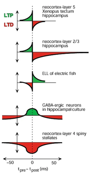
With that said, the pre before post shape is the one we’re normally talking about, and that what we’ll focus on in this section.

Modelling STDP¶

So how do we model this? The simplest thing would be just to start with the single pair weight change:

Then sum the weight change over all spike pairs.

The issue is that this is computationally expensive. Suppose we have $N$ neurons all-to-all connected to $N$ neurons, and each neuron fires around $R$ spikes. In that case, computing this sum takes around $N^2$ $R^2$ operations, and each operation contains a call to the exponential function which is itself very heavy.

There is a trick that can simplify this, using the fact that it’s exponentials and linear sums. For each pre-synaptic neuron we introduce what is called a trace variable, $a_{\pre}$. We do the same with the post-synaptic neurons and a trace variable $a_{\post}$.

We update them according to the following rules. In the absence of a spike, they decay exponentially like we’ve seen in the leaky integrate-and-fire neuron. The pre-synaptic trace with time constant $\tau_+$ and the post-synaptic with time constant $\tau_-$.

When a pre-synaptic spike arrives:

And similarly for a post-synaptic spike arrives but with pre and post swapped and + and - swapped.

Computationally, we now only have to do $O(N^2 R)$ operations, and they’re all arithmetic instead of exponential. This is essentially free because we had to this many operations anyway. For each spike at a pre-synaptic neuron, we have to add a value to each post-synaptic neuron it’s connected to. There are $N$ neurons affected by each spike, and there are $NR$ pre-synaptic neurons, so that’s $N^2 R$ operations we would have had to do anyway.

One thing that’s worth pointing out is that the models slightly differ from the experimental data here. In the experimental data, it takes around an hour before you see the weight change, with it slowly increasing over time. With the first implementation, we could run the weight change rule an hour after the spikes we want to learn, but even that doesn’t match the slow change you see in experiments. With the second implementation, it’s automatically updated immediately after each spike.

It’s also worth noting that there are some subtleties with delays here. You should do a slightly different thing depending on whether the delays are dendritic, axonal, or some combination of the two. In any case, the experimental data is less clear about delays, so it’s not even obvious that there is a right thing to do here.

Latency reduction¶

Now that we know how to model STDP, let’s start taking a look at the things it can learn. Let’s start with a result from Song et al. (2000).

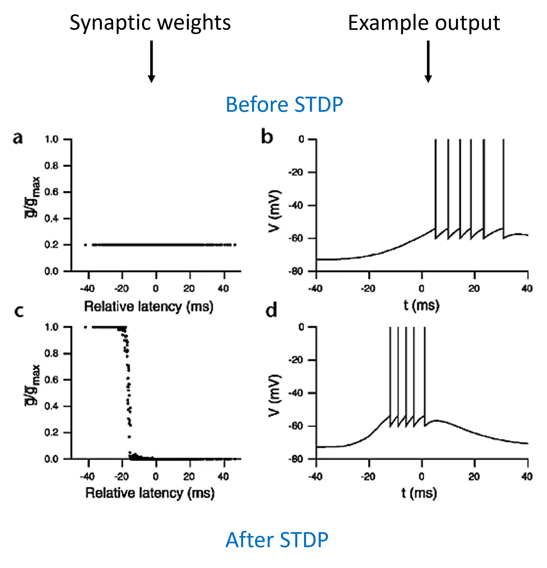
We set up a model with a layer of input neurons connected to a single output neuron, with STDP on the synaptic weights. Now, we make those input neurons all fire a burst of spikes for 20 ms but with a random latency, and look at what the network learns.

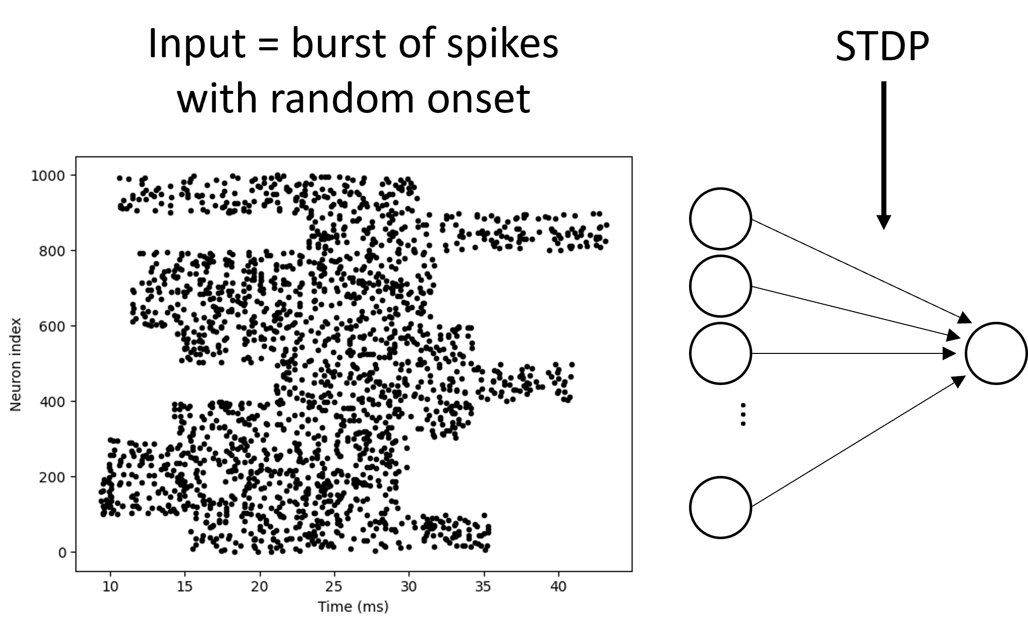
What we see is that the neurons with a low latency have their synaptic weights strengthened to the maximum level, and those with a high latency drop to zero. The output neuron now spikes earlier than before learning. One way of interpreting this would be that if there were multiple sources of information available to an animal, it would respond preferentially to the one that arrived earliest. This would clearly be advantageous in an environment where a short delay in responding could be the difference between life and death for an animal being hunted.

STDP learns correlated groups¶

In this next experiment Song & Abbott, 2001, we divide input neurons into two groups. One group with the white background are firing uncorrelated spikes. The other group with the blue background are firing correlated spikes.

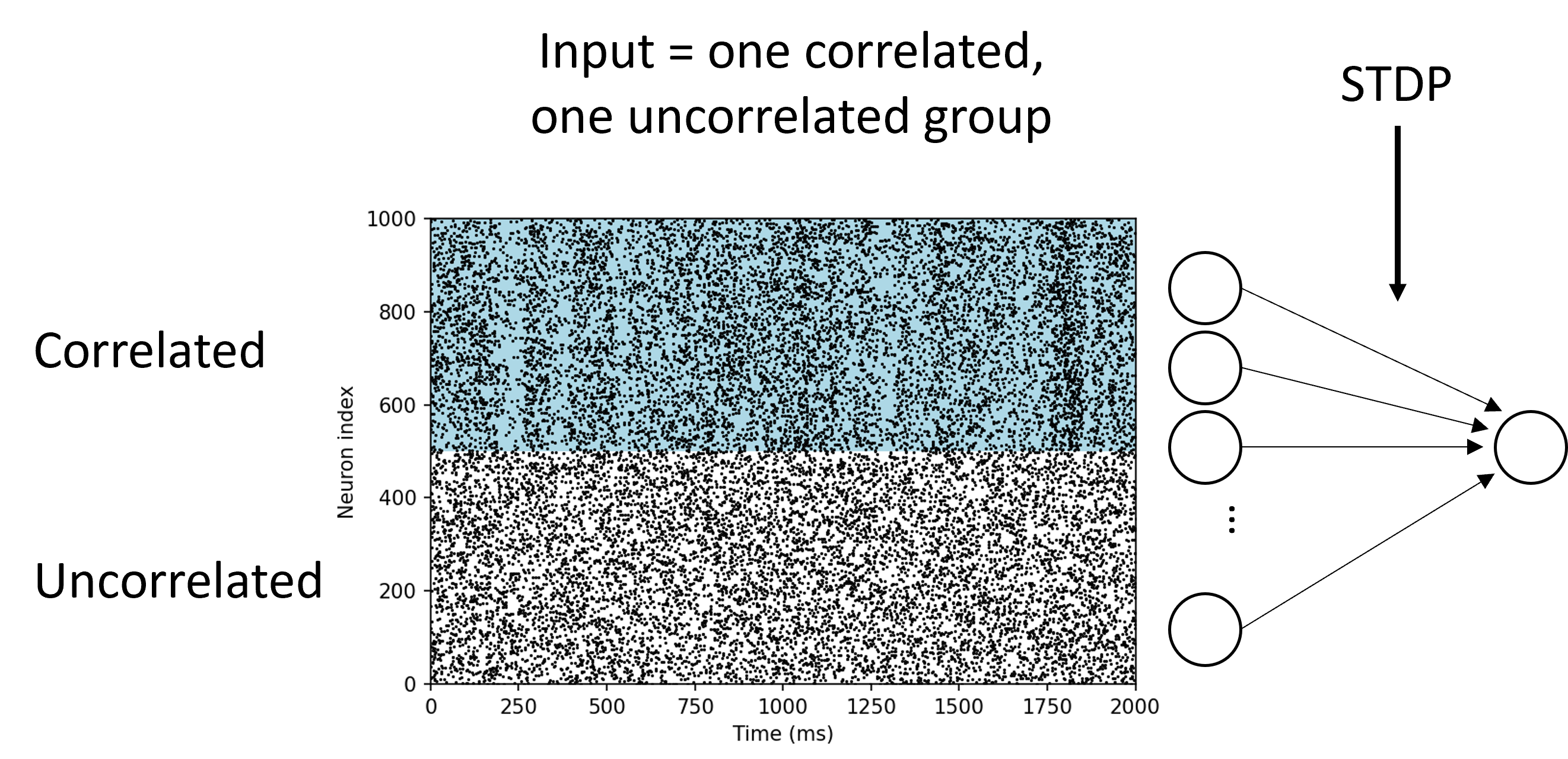
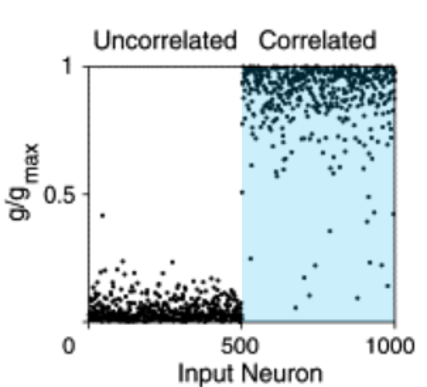
After STDP, the weights of the neurons in the uncorrelated group go to zero, while the weights in the correlated group go to the maximum value. This makes sense biologically because being able to pick up on input correlations in your environment is very useful.

We can do the same thing but where both groups of neurons are correlated with other neurons in their group, but not with neurons in the other group. We find that STDP will learn to pick one of the two groups, but which one is random. In other words, STDP has some aspects of competition in what it learns. You can think of this as a bit like the selectivity we talked about with the BCM rule in the previous section.

STDP finds the start of spike sequences¶

The next model Masquelier et al., 2008 combines the ideas from these two previous papers to learn to respond to repeated sequences of spikes. We have the same setup with a group of neurons connected via STDP synapses to a single output neuron. In this case, the input is random, uncorrelated spikes that have repeated patterns repeated at random times. The blue dots are the uncorrelated spikes, and the red dots are the repeated patterns.

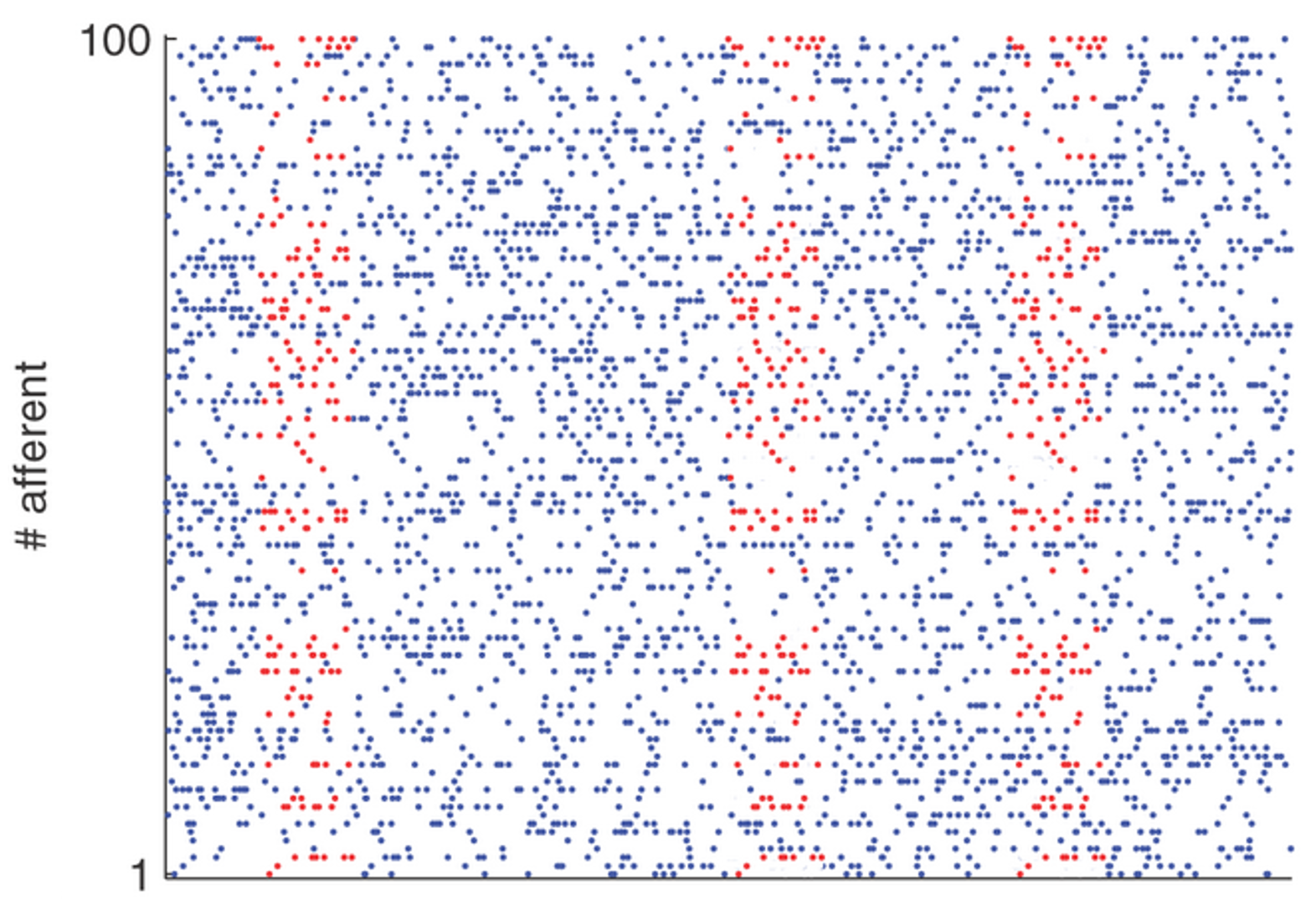
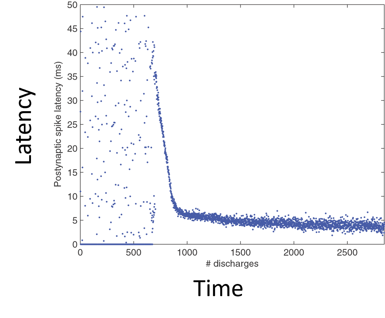
What happens here is that the output neuron initially fires at random times, but eventually learns to fire only when the spike pattern is present. In fact, it learns to fire at the start of spike pattern

If you look more carefully, at first it learns a random subset of the neurons in the spike pattern group that happen to fire at the same time. This is the correlation and competition mechanism from the previous slide, and it leads to the output spike happening at some random point in the sequence: could be early, could be late. Then, STDP’s preference for lower latency kicks in, and it shifts towards the neurons in the pattern that fire earlier, until it reaches the beginning.

A later study Agus et al., 2010 found that humans can indeed learn random patterns in noise. Specifically, what they did was to play pairs of bursts of random noise to human listeners, and they had to indicate whether it was the same noise burst repeated, or two different ones. Unknown to them, sometimes the repeated bursts of noise were the same as ones they had heard before. The result was that listeners learnt to recognise repeated bursts of noise more accurately for the ones they had heard before than for fresh bursts of noise, even though all the bursts were entirely meaningless samples of white noise.

STDP learns spatial maps¶

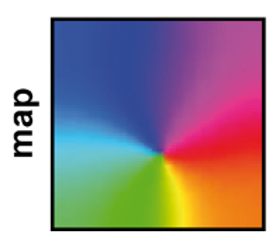
In week 2’s network models, we saw the example of a spatial map in the barrel cortex of the rat. As a reminder, that’s the system that processes inputs from the rat’s whiskers. What we saw is that these neurons have a preference for motion in a particular direction, and that preference has a spatial structure.

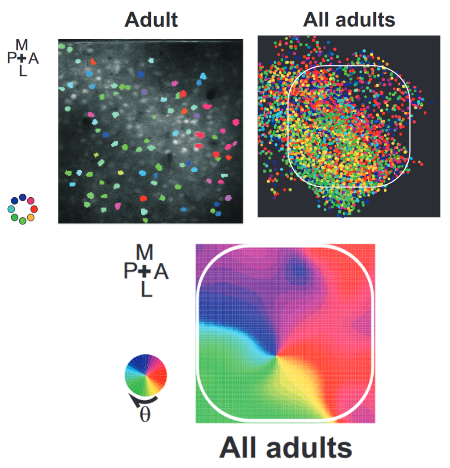
To model this Kremer et al., 2011, we used a slightly more complicated setup than the previous studies, designed to match the structure of layers 2 through 4 of the barrel cortex. The input stimuli were waves of activity that moved across the whiskers in a linear pattern, with the direction chosen randomly each time.

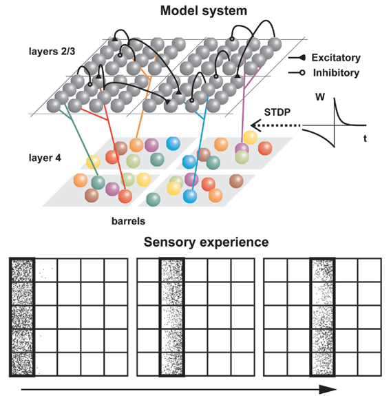
This input structure together with the STDP synapses was enough for the model to learn a very similar input selectivity map to what was recorded in the rats.

Issues with STDP¶

So STDP is pretty cool and can learn some fun stuff, but there are some problems too.

Saturation¶

We saw in the section on rate-based models that without some careful control, weights tend to go to the extremes and earlier in this section you could see the same thing happening with STDP - the weights all push towards the maximum or minimum allowed values.

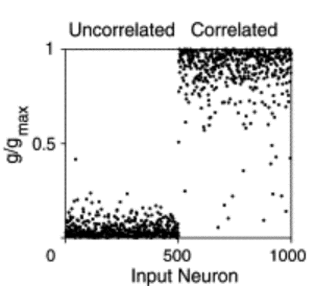
This doesn’t match what you see experimentally.

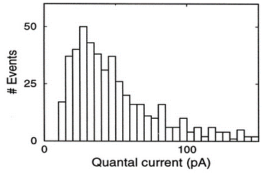
You can fix this with a noisy, multiplicative version of the STDP learning rule Rossum et al., 2000, although it’s harder to get strong competition and specialisation with this form of STDP.

Bidirectional pairs¶

Another issue is that STDP will always force synaptic connections between neurons to be unidirectional. You can’t have a situation where A excites B and B excites A. However this is common in cortex.

You can fix this with a more complicated STDP rule that takes voltage into account Clopath et al., 2010, and the properties of these sorts of models are still being investigated. It is structurally similar to the BCM rules we saw in the last section, and also gives rise to selectivity and something like independent component analysis.

Stability across time scales¶

A more fundamental problem that has not yet been solved is how to handle stability of learning across multiple time scales. Yger & Gilson (2015) has a nice review of many models from a dynamical systems point of view, showing that when you combine different forms of learning at different time scales, all sorts of problems start to occur like oscillations that disrupt memories.

In general, we know that it’s important to combine multiple time scales because we want to be able to learn fast and forget slowly, but this seems to be hard to achieve. This is related to the similar problem of catastrophic forgetting found in machine learning, and solutions to this problem in either neuroscience or machine learning may prove helpful in the other field.

Other issues¶

This isn’t a complete list of all the issues with STDP, and if you’re interested in taking it further Shouval (2010) has quite a nice review of some of the problems and attempted solutions.

Other forms of learning¶

OK, that’s the end for this week on learning rules. There’s a lot more stuff that could be covered here, and that we might add later. In case you’re interested, there are some key words to look up to take it further.

This includes reward modulated STDP that lets you combine STDP with rewards to learn more interesting tasks.

There’s reservoir computing that applies a linear readout layer to a random network with or without STDP, and turns out to be capable of learning arbitrarily complex functions with some assumptions.

There’s the famous Hopfield network and associative memory.

Of course, there’s reinforcement learning.

And many, many more!