Introduction
In this section we’re going to start looking at modelling networks, which in some sense is the topic of the rest of the course.
A key question we might want to answer is: what can networks do that single neurons can’t?
The simple answer is that they can do anything, which makes it tricky to decide what to include in a short section like this. Let’s first unpack what we mean by that.
Universal function approximation
From the History of neuroscience and machine learning section, you’ll know that as early as 1943 McCulloch and Pitts showed that spiking neural networks could implement any logical function. And we don’t need to limit ourselves to logical functions.
Just as for artificial neural networks, spiking neural networks are universal function approximators. That is, they can approximate any reasonable function. This has been proven in various ways by different people over the years, but we’re going to highlight a particularly nice and simple proof by Iulia Comșa at Google Research.
Her paper Comsa et al., 2019 starts by showing that you can implement the less than and greater than operators using spiking neurons. We’ll do a similar thing in this week’s exercise.
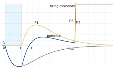
Figure 1:Implementing comparative operators using spiking neurons Comsa et al., 2019.
Next, by adding in a network that implements logical-AND, you can express intervals or, in higher dimensions, hypercubes.
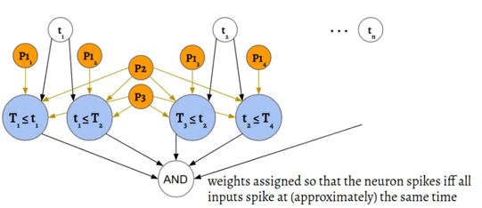
Figure 2:Implementing logical AND Comsa et al., 2019.
Finally, by combining these you can approximate any function to as much accuracy as you want by just dividing into smaller and smaller hypercubes.
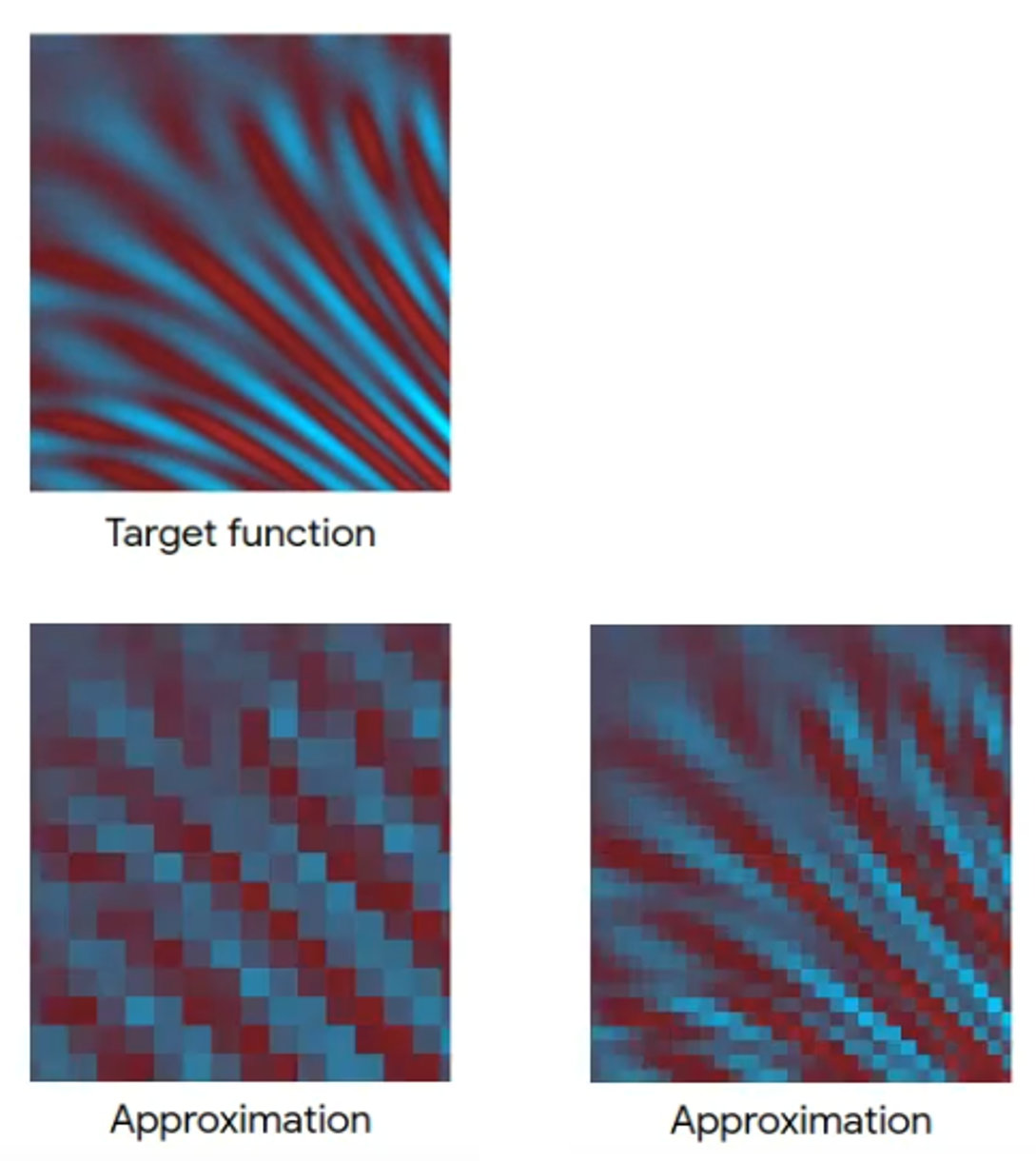
Figure 3:Function approximation via hypercube division Comsa et al., 2019.
So that’s great and perhaps not unexpected given that our brains are just spiking neural networks, and we like to think we’re fairly capable.
But it does mean that there’s no way we can cover all the things we can do with networks.
So instead, what we’re going to go through, in detail, is one particular type of network, and show how it ties in to some of the concepts that neuroscientists use to understand the brain.
Sound localisation circuit
The circuit we’ll look at is the sound localisation circuit.
One of the key ways we can tell which direction a sound is coming from is because there’s an arrival time difference of the sound between the two ears.
Depending on head size and the angle the sound is arriving from, for humans this is a maximum of around 650 microseconds, we’re able to discriminate sounds arriving with a time difference as small as 20 microseconds.
Some animals like owls can discriminate differences as small as just a few microseconds. So how can we detect this?
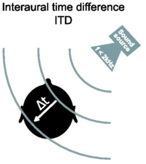
Figure 4:Detecting where sound is coming from using difference in arrival time between two ears Grothe et al., 2010.
One model is due to Lloyd Jeffress in 1948 and still found in textbooks, although the reality is a bit more complicated as we’ll see.
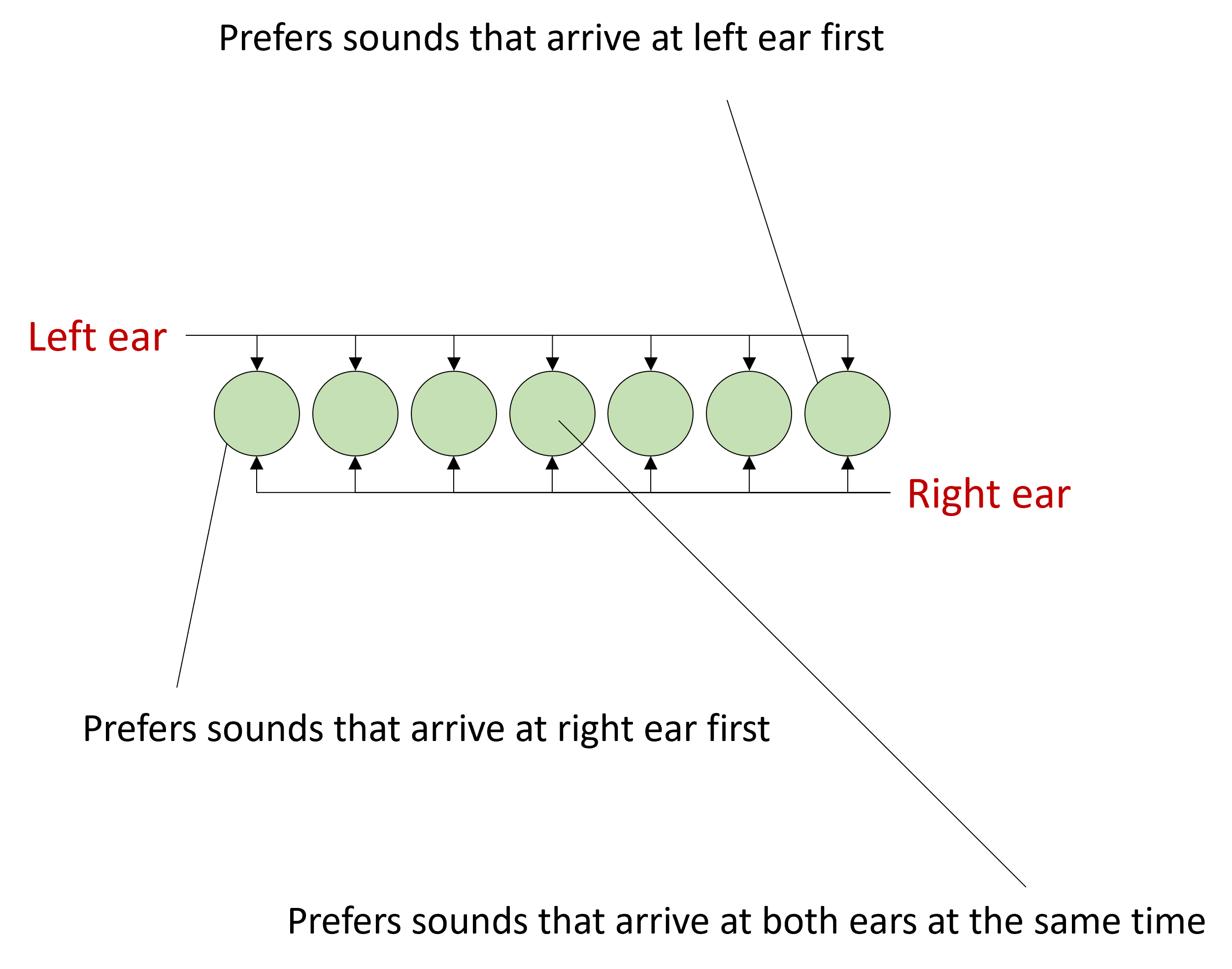
In his model, you have an array of what are sometimes called coincidence detector neurons.
These are neurons that will only fire a spike if they receive a simultaneous input from both their synapses.
The signal arrives from the left ear, and travels at constant speed along this pathway, arriving at each neuron with a slightly different delay.
At the same time, the signal arrives from the right ear and does the same thing but in the reverse direction. When the acoustic delays exactly cancel with the neural delays, the signal will arrive at the coincidence detector at the same time and cause it to spike, and we can use the identity of which neuron fired a spike to tell us where the sound came from.

In this example, you can see that the sound arrives first at the left ear in the third window, and then in the right ear in the 5th window, so there’s a 2 window time difference. When the sound happens, the signal will appear at the left and start to move right, and then at the right move left. They arrive at the relevant cell at the same time causing it to light up.
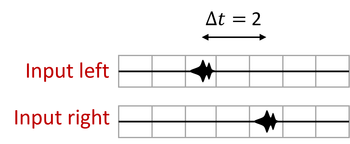
So that’s how Jeffress’ model of sound localisation works, and it has a few interesting and more general features that we can dig into.
Coincidence detection and tuning curves
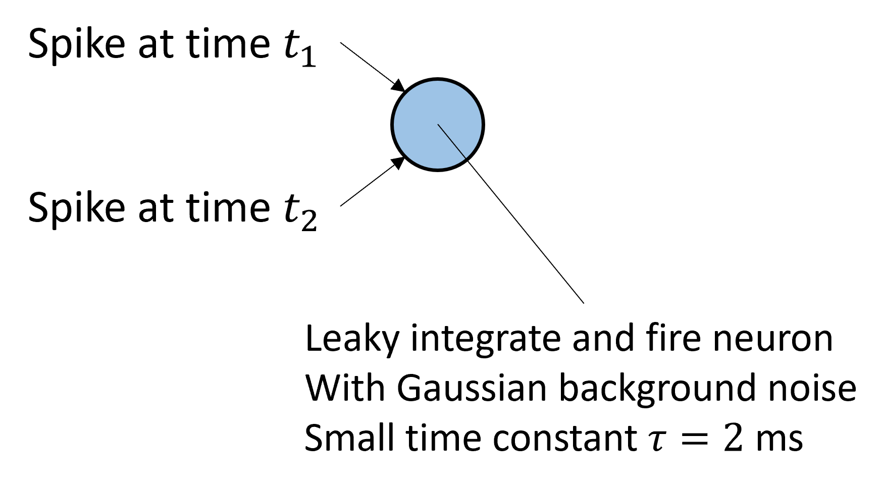
The first feature is coincidence detection. It’s actually quite a general property of leaky neurons, precisely because of the leak, as you can see in this picture. When two spikes arrive at similar times, they’re enough to drive the neuron over threshold and cause a spike. Whereas when they arrive with a larger time difference, the leak between the spikes means the peak is lower and not enough to drive it over threshold.

We can plot the effect of this on a neuron that receives two spikes, and to make it a bit more realistic, a fluctuating, Gaussian background noise.
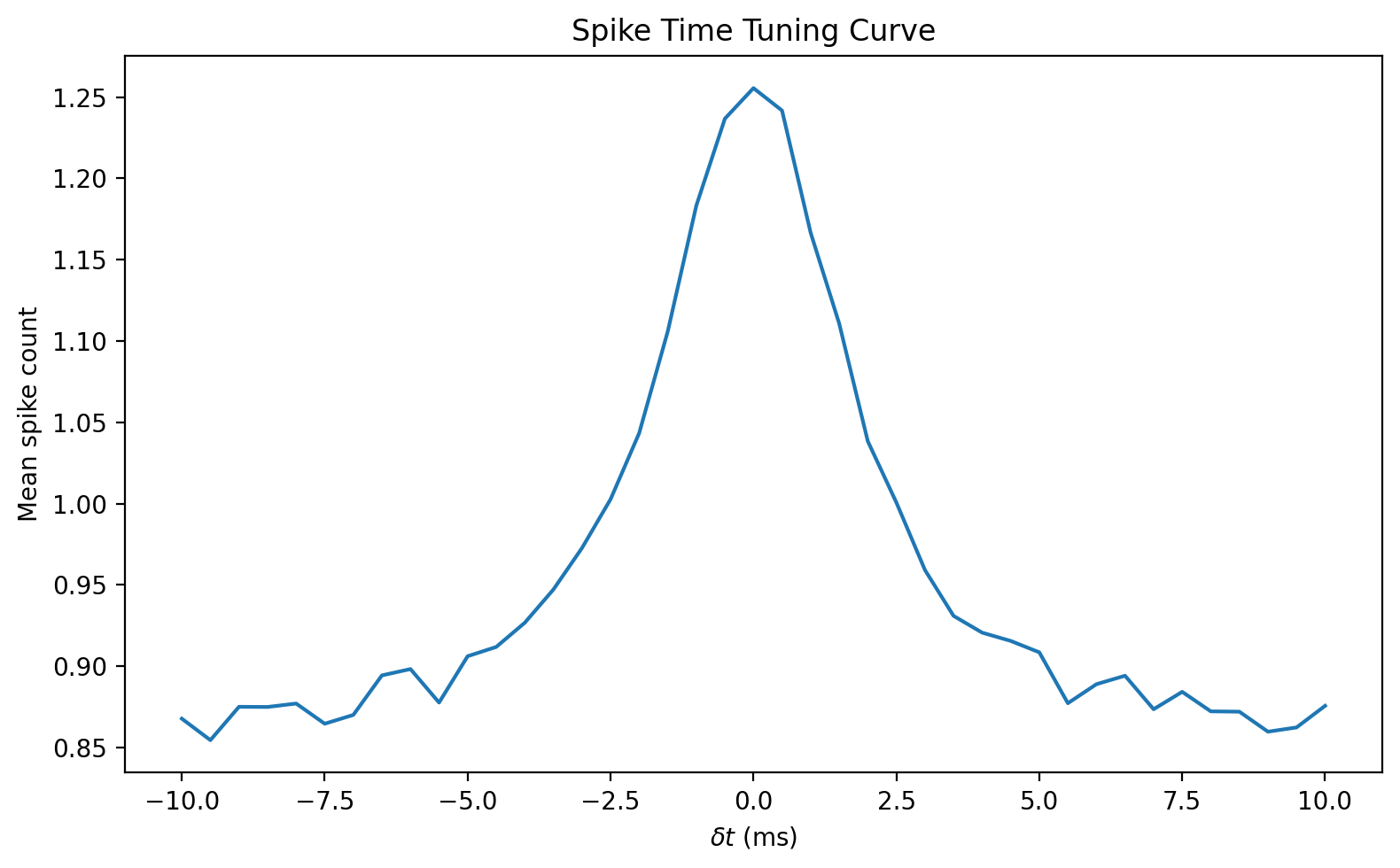
On the graph, you can see that the neuron fires more spikes when the arrival time difference between the spikes is smaller - precisely what we want.
This is one example of what’s called a tuning curve in neuroscience. It shows the response of a neuron, averaged over several repetitions, to a stimulus defined by one or more variables.
In this case, the variable is the arrival time difference between the two spikes, but it could be anything, like the contrast of a visual image, the amplitude or pitch of a sound etc. It can also be 2D in which case you’d plot it as an image. We’ll come back to tuning curves a bit later.
Spatial structure
Another aspect of this network that you see many times in neuroscience is the spatial structure. The cells here are in a 1 dimensional array in order of their preferred difference in arrival time. You see this sort of pattern in 1D and 2D across the brain in auditory, visual and other modalities.
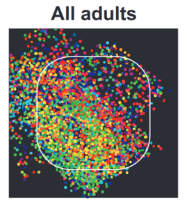
Here’s an example from the barrel cortex of the rat. That’s the part of the brain that processes inputs from the rats’ whiskers. The coloured blobs shows the preferred stimulation direction of the cell recorded at that position. The spatial structure isn’t obvious because there are so few cells recorded.
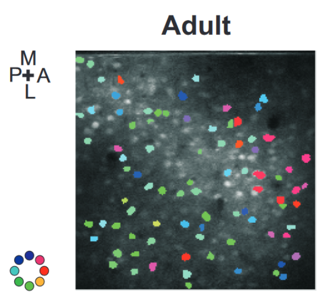
Figure 9:Direction preferences of cells in the barrel cortex of a rat Kremer et al., 2011.
But, you start to see it if you combine across multiple animals.
And with a bit of smoothing it becomes even clearer.
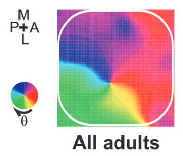
One interesting feature of this is that it’s learned, as you don’t see this in young rats, only adults.
In terms of modelling, it’s fairly easy to just add some metadata to each neuron specifying its position, and use that in your models. For example, you could use that to make connections between nearby neurons more likely than between neurons that are far away.
Encoding and Decoding
With the idea of tuning curves and spatial structure in mind, we can talk about how information is encoded and decoded in this network.
Essentially, the model Jeffress proposed is what we would now call a 1-hot encoding. Knowing the identity or index of the most active neuron tells you the category of the data. In this case, a value put into one of several discrete intervals.
More recently, it was noted that in the presence of neural noise, this isn’t a very robust way of decoding that information.

Grothe et al. (2010) proposed an alternative view of what the brain might be doing to decode information from this network.
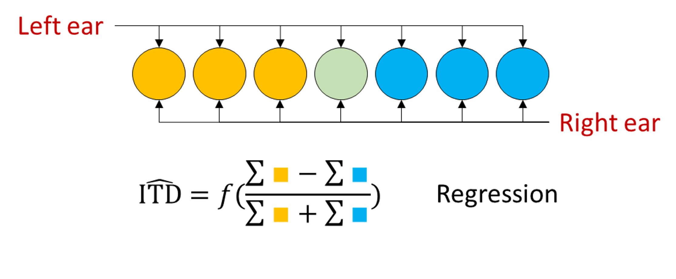
Their idea was to take the difference of the summed activities of the cells that prefer right leading sounds to those that prefer left leading sounds, and to use this 1d variable to regress the location.
It turns out this is much more robust to noise. Conceptually, this is because by summing or equivalently averaging all the activity of the cells, you reduce the effect of noise.
In 2013, Dan wrote a paper which can be summarised by saying that you can do better than either of these approaches by using a standard multi-class perceptron Goodman et al., 2013. This makes use of all the information in a way that neither of the other two models does, including averaging out the noise.
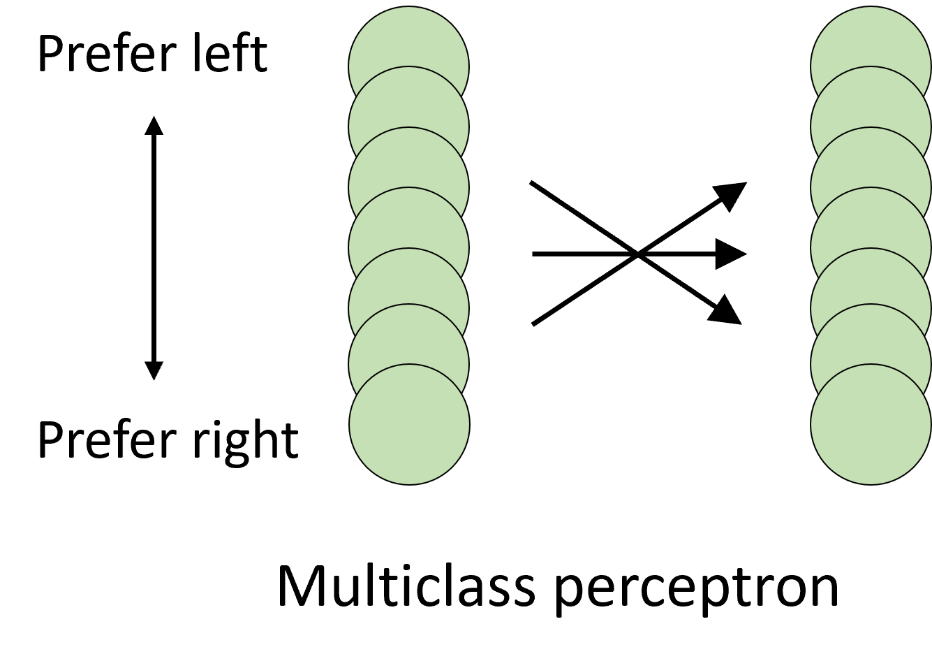
In one of those strange twists of fate, the same year Dan’s paper came out, another paper Day & Delgutte, 2013 came out from the lab Dan had just moved to that was basically the same, only they used a Bayesian decoding framework rather than perceptrons, and so we’ll use their paper to talk about that framework.
Maximum likelihood and Bayesian estimators
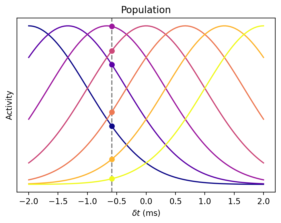
We’ve seen how we have an array of coincidence detectors whose response is larger or smaller depending on the arrival time difference of the sound. Now imagine we plot all the tuning curves on top of each other for this population of neurons.
If the ITD were where the grey vertical line is, then we’d see the responses at the circles shown on the graph below, and the idea is to use that pattern of responses to work out the ITD.
If there were no noise, you could just read it out easily from this figure, but these responses are very noisy, so we have to use a probabilistic method.
There’s one very common way to do that.
We want to estimate the ITD θ.
We know the neural responses as a vector of responses of units .
We assume they’re independent so we can easily compute the probability of a given vector of responses given a value of theta as the product of the probabilities of each individual response:
Then our maximum likelihood estimator is the value of θ that makes the observed response the most likely:
But we don’t know this probability of θ given , only the reverse, .
That’s where Bayes’ theorem comes in because it lets us calculate one in terms of the other:
In particular, since we’re computing an argmax over θ, we can ignore any term that doesn’t depend on θ, so we can ignore the term.
If we assume that all values are equally likely we can also ignore the term. If instead we have a prior of which ITDs are more likely than others, we can incorporate this here and then the method is known as maximum a posteriori or MAP estimation.
Now we can express the estimate we want in terms of things we can calculate:
That all seems quite abstract, but in this case if we can make some additional assumptions which simplifies things nicely.
Let’s assume the shape of the tuning curves is approximately Gaussian, centred on some preferred ITD . We also assume that the noise is Poisson distributed (which is a reasonable model). With these assumptions, the maximum likelihood estimator simplifies to an average of the preferred ITDs, weighted by the responses. That was a very quick run through probabilistic population coding.
For more
We’d recommend the theoretical neuroscience textbook by Dayan and Abbott (free pdf), or since that’s out of print, a more recent book “Bayesian models of perception and action” by Wei Ji Ma and colleagues, available free online.
Single neuron and Population Sensitivity
OK that’s pretty much it for the sound localisation example, we just wanted to finish by highlighting what we’ve gained from the network here.
A single neuron has a time sensitivity controlled by its time constant, at the smallest around one millisecond. And it has a lot of noise.

We’ve seen this curve, but that’s an average over ten thousand repetitions.

On a single trial it looks like this. Unlikely we could make a very accurate estimate from that.
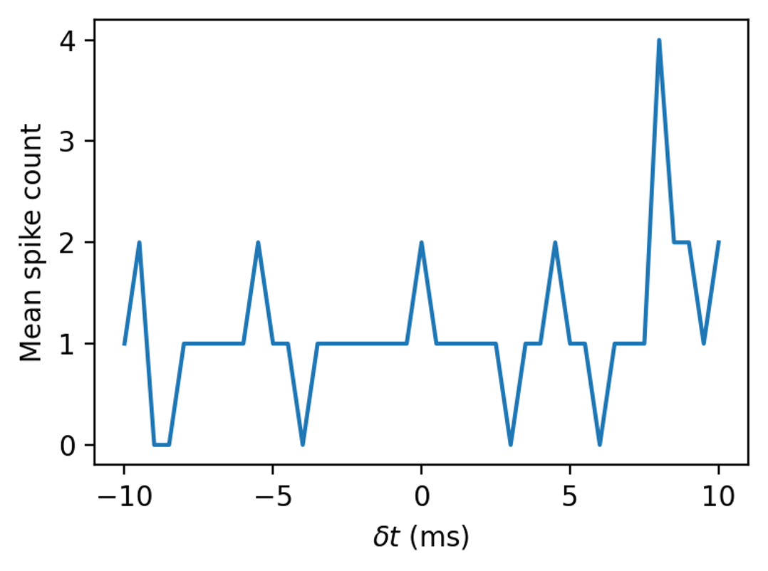
By switching to a population and using a population level decoder we get a system that is sensitive to time differences of a few microseconds. Orders of magnitude more time sensitive than the speed of the fastest units in the network.
Various topics
We can’t cover everything about networks here, so to finish off we just want to highlight two interesting things you might want to read up on further.
Balanced excitation/inhibition
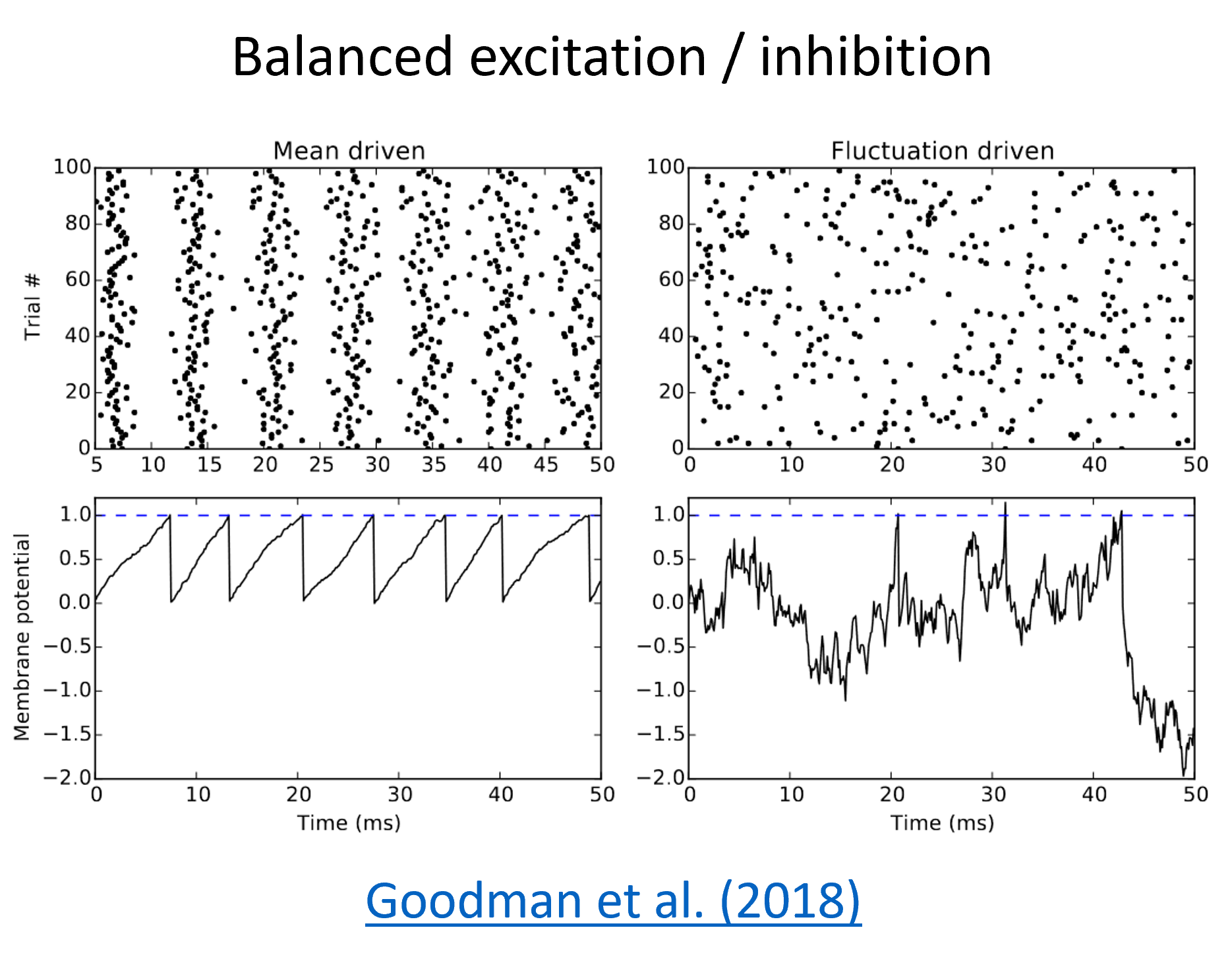
Cortical neurons receive thousands of tiny inputs per second, so why don’t they all fire very regularly like on the left of this figure?
One possible answer is that there is a balance of excitation and inhibition, and if excitatory and inhibitory inputs are balanced and randomly interspersed, a neuron can fire very irregularly. You can see the effect of that on the right.
You actually see both types of behaviour in the brain, and having a range of such behaviours might be important. In Goodman et al. (2018), Dan looks at different mechanisms that can contribute to that in the early auditory system.
More generally, some of the possible roles that have been suggested for balanced excitation/inhibition include improving the sensitivity, noise robustness and response speed of a network. There’s a big literature on this.
Central pattern generators
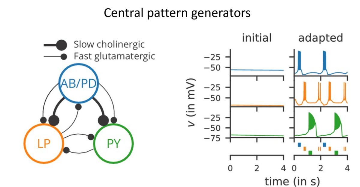
Another fascinating thing is central pattern generators. These are small networks that seem to just emit the same pattern of spikes on repeat forever. They’re thought to be involved in coordinating movements, basically providing a regular signal that can be transformed into stereotypical sequences that we need to move our muscles in standard patterns.
Some of the circuits for this can be very simple, like this one shown schematically here in the lobster stomatogastric ganglion. This one is particularly interesting because it was found in modelling studies that there were many different parameters for this circuit that give the same output. And then later it was found experimentally that this is also the case in real lobsters: different individuals can have widely different neural properties in this circuit and still it functions in the same way. We’ve put more reading on this topic and the others in this section in the reading list. Also, we will be coming back to some other networks topics like memory and decision making later in the course.
- Comsa, I. M., Potempa, K., Versari, L., Fischbacher, T., Gesmundo, A., & Alakuijala, J. (2019). Temporal Coding in Spiking Neural Networks with Alpha Synaptic Function: Learning with Backpropagation. arXiv. 10.48550/ARXIV.1907.13223
- Grothe, B., Pecka, M., & McAlpine, D. (2010). Mechanisms of Sound Localization in Mammals. Physiological Reviews, 90(3), 983–1012. 10.1152/physrev.00026.2009
- Kremer, Y., Leger, J.-F., Goodman, D., Brette, R., & Bourdieu, L. (2011). Late Emergence of the Vibrissa Direction Selectivity Map in the Rat Barrel Cortex. Journal of Neuroscience, 31(29), 10689–10700. 10.1523/jneurosci.6541-10.2011
- Goodman, D. F., Benichoux, V., & Brette, R. (2013). Decoding neural responses to temporal cues for sound localization. eLife, 2. 10.7554/elife.01312
- Day, M. L., & Delgutte, B. (2013). Decoding Sound Source Location and Separation Using Neural Population Activity Patterns. The Journal of Neuroscience, 33(40), 15837–15847. 10.1523/jneurosci.2034-13.2013