Synapse models - Neuroscience for machine learners

Introduction¶

In the last section we went through a lot of detailed biology! In this section we’re going to turn that detailed biology into relatively simple equations.

Level of abstraction¶

Previously we explained how when a spike arrives at a transmitting synapse, a neurotransmitter is released. This neurotransmitter causes a change in the conductance of the receiving cell due to the opening of an associated ion channel.

In turn, this leads to an input current following the same sort of equations we saw for the Hodgkin-Huxley formalism last week. This then leads to a change in membrane potential for either the Hodgkin-Huxley or leaky integrate-and-fire type neurons. Just as we did for neurons, we need to decide what level of detail we want to include in our synapse model.

One reason we might want to leave out some of this detail is that some of these changes will happen fast enough that modelling their temporal dynamics won’t change much at the scale we’re looking at.

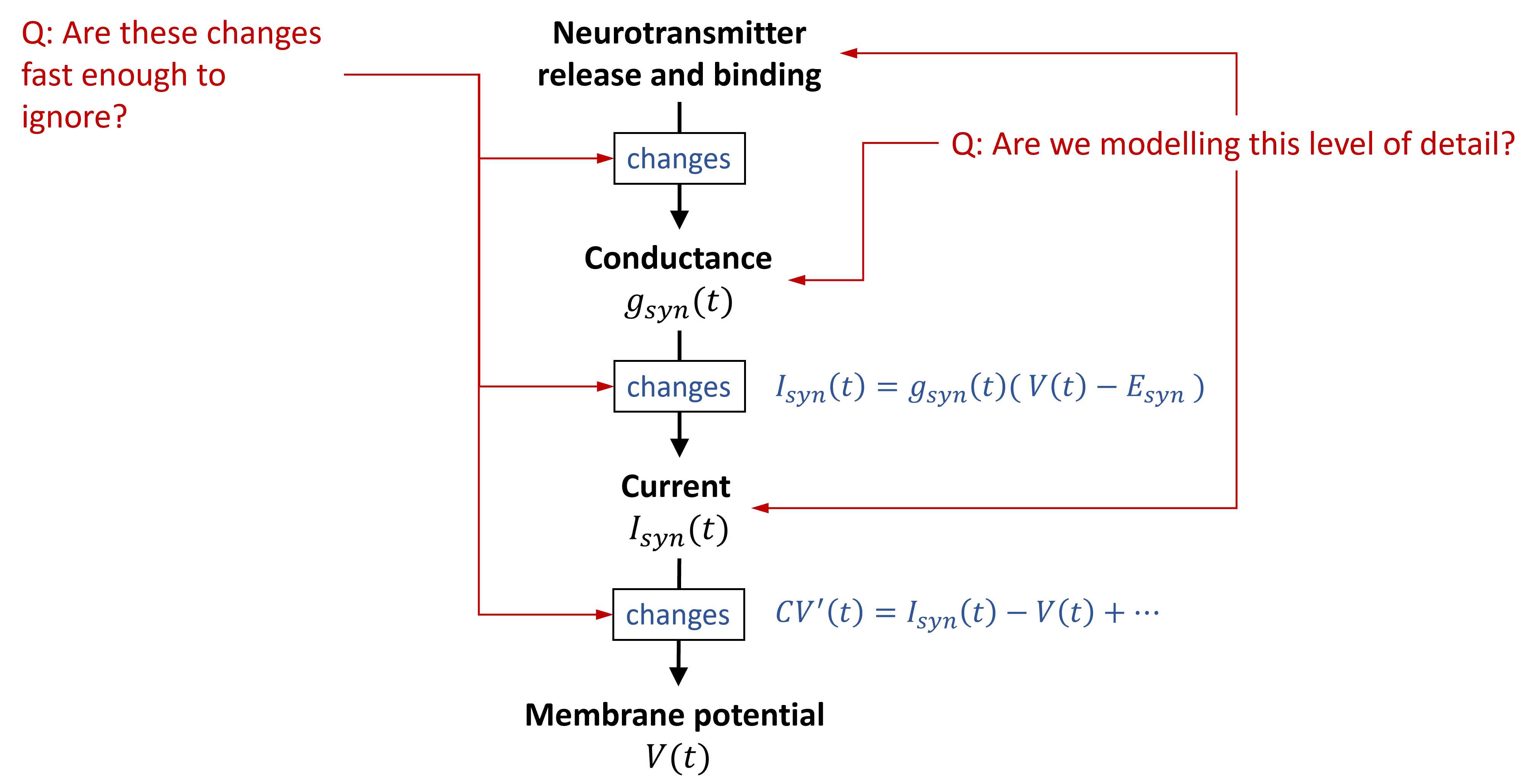
Figure 1:Deciding on the right level of abstraction for synapse models.

A helpful picture to draw is the postsynaptic potential, sometimes referred to simply as a PSP (shown below). This shows the increase in the membrane potential of the receiving cell as a result of a spike arriving at that cell. In this figure you can see a model synapse at three levels of detail:

Blue - instantaneous increase in the membrane potential
Orange - instantaneous increase in a current, which then decays exponentially back to rest
Green - instantaneous increase to the conductance.

Source:

💻 Code for figures

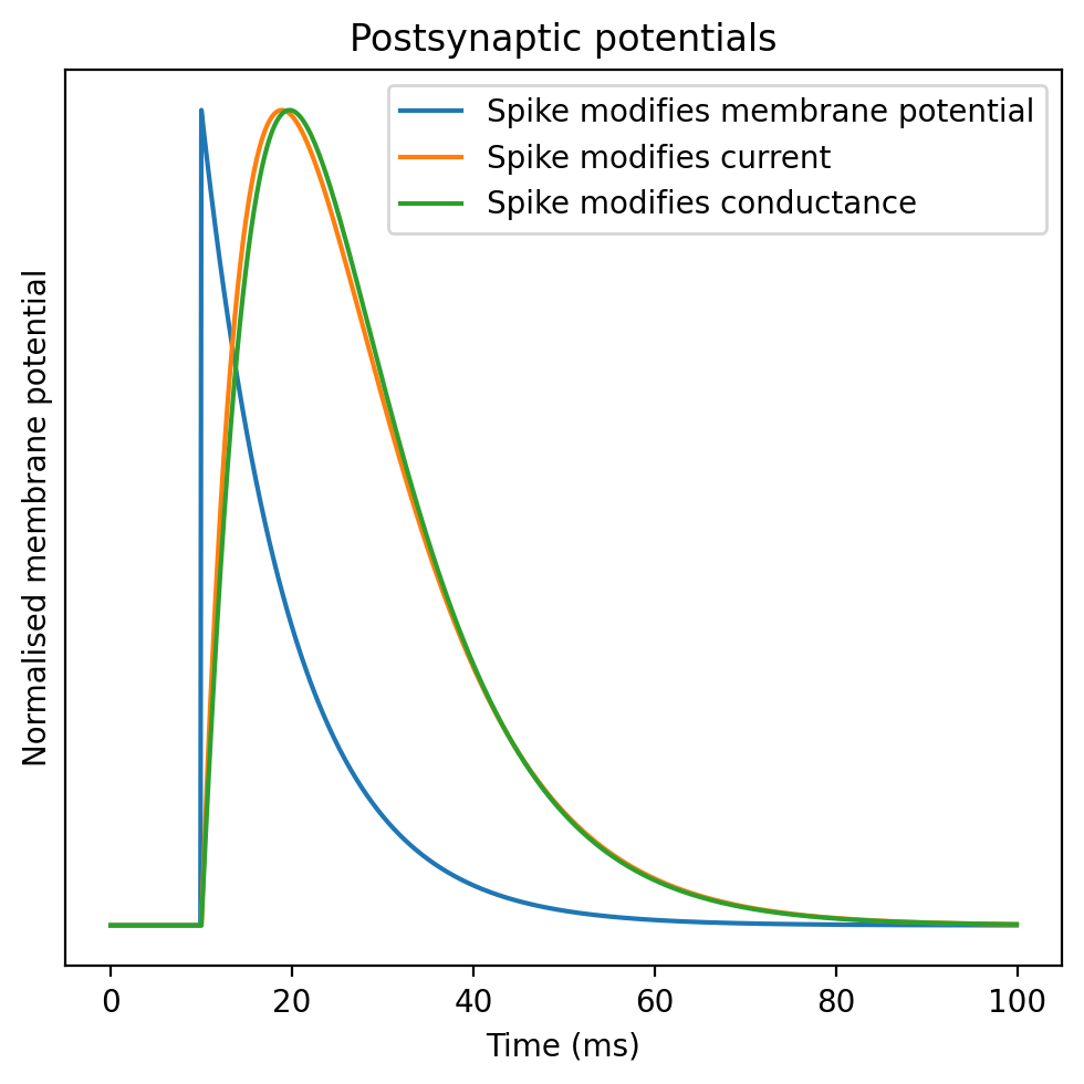
Synapse time course¶

We will start with how we can directly model the dynamics in terms of conductance, current or membrane potential. A common approach is to decide the key synaptic variable and model it with one of the three classes of functions. There’s an explanation as to why these three classes come up that we’ll return to later.

For simplicity, we’ll describe each of these as postsynaptic membrane potentials, although they can also be used to model currents or conductance.

The fist case is the exponential function which can be written as the product of an exponential decay with some time constant and a Heaviside function.

v(t) = H(t)e^{-t/\tau}

(1)

Source:

💻 Code for figures

A step-up in complexity is the alpha function which we haven’t seen before. In this equation, we multiply the exponential decay by t so that it rises continuously before decaying.

v(t) = H(t)e^{-t/\tau}t/\tau

(2)

Source:

💻 Code for figures

A further step-up is the biexponential function, which lets us seperately control the rise and fall time with 2 different time constraints.

\begin{aligned} v(t) &= H(t)(e^{-t/\tau} - e^{-t/\tau_x}) \\ \tau_x &\neq \tau \end{aligned}

(3)

Source:

💻 Code for figures

Each of these can be represented as a linear time invariant differential equation with constant coefficients. This makes sense since we would expect time invariance in a model of a physical system. Having linearity and constant coefficients is the simplest thing we can do.

ODE for exponential form:

\begin{aligned} \tau v' &= -v \\ v(0) &= 1 \end{aligned}

(4)

ODE for alpha form:

\begin{aligned} \tau v' &= x-v \\ \tau x' &= -x \\ x(0) &= 1 \end{aligned}

(5)

ODE for biexponential form:

\begin{aligned} \tau v' &= x-v \\ \tau_x x' &= -x \\ x(0) &= 1 \end{aligned}

(6)

We can take this argument further by putting these equations into matrix form and calculating their eigenvalues.

Matrix form for exponential form:

\begin{aligned} \boldsymbol{y} &= (v) \\ M &= (-1/\tau) \\ \text{Single eigenvalue} &= -1/\tau \end{aligned}

(7)

Matrix form for alpha form:

\begin{aligned} \boldsymbol{y} &= (v,x) \\ M &= \begin{pmatrix} -1/\tau & 1 \\ 0 & -1/\tau \end{pmatrix} \\ \text{Repeated eigenvalue} &= -1/\tau \end{aligned}

(8)

Matrix form for biexponential form:

\begin{aligned} \boldsymbol{y} &= (v,x) \\ M &= \begin{pmatrix} -1/\tau & 1 \\ 0 & -1/\tau_x \end{pmatrix} \\ \text{Two eigenvalues} &= -1/\tau, -1/\tau_x \end{aligned}

(9)

These three forms are essentially the only possibilities for a 1 or 2-dimensional system that is linear, time invariant and has constant coefficients. The exponential is the only possibility for 1 dimension, and in 2 dimensions you either get the alpha or biexponential depending on whether the eigenvalue is repeated (see box below).

Short-term plasticity¶

So far we’ve looked at memoryless models of synapses, where previous activity doesn’t affect what they do, but this isn’t quite right. Neurotransmitters are released in vesicles, and after being released, a fraction of them will be unavailable if another spike comes along. This means that later spikes will likely have a smaller effect than earlier spikes. This is called short-term synaptic depression. We can model it by adding an extra variable $x$ that tracks what fraction of vesicles are available.

Source:

💻 Code for figures

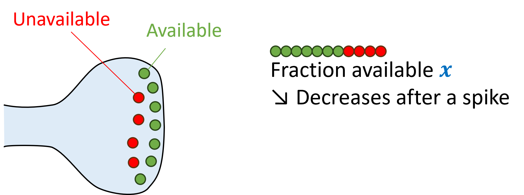
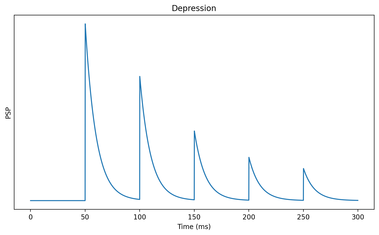
However, it turns out that you also see cases where each subsequent spike has a bigger effect than previous spikes, which is called facilitation.

Source:

💻 Code for figures

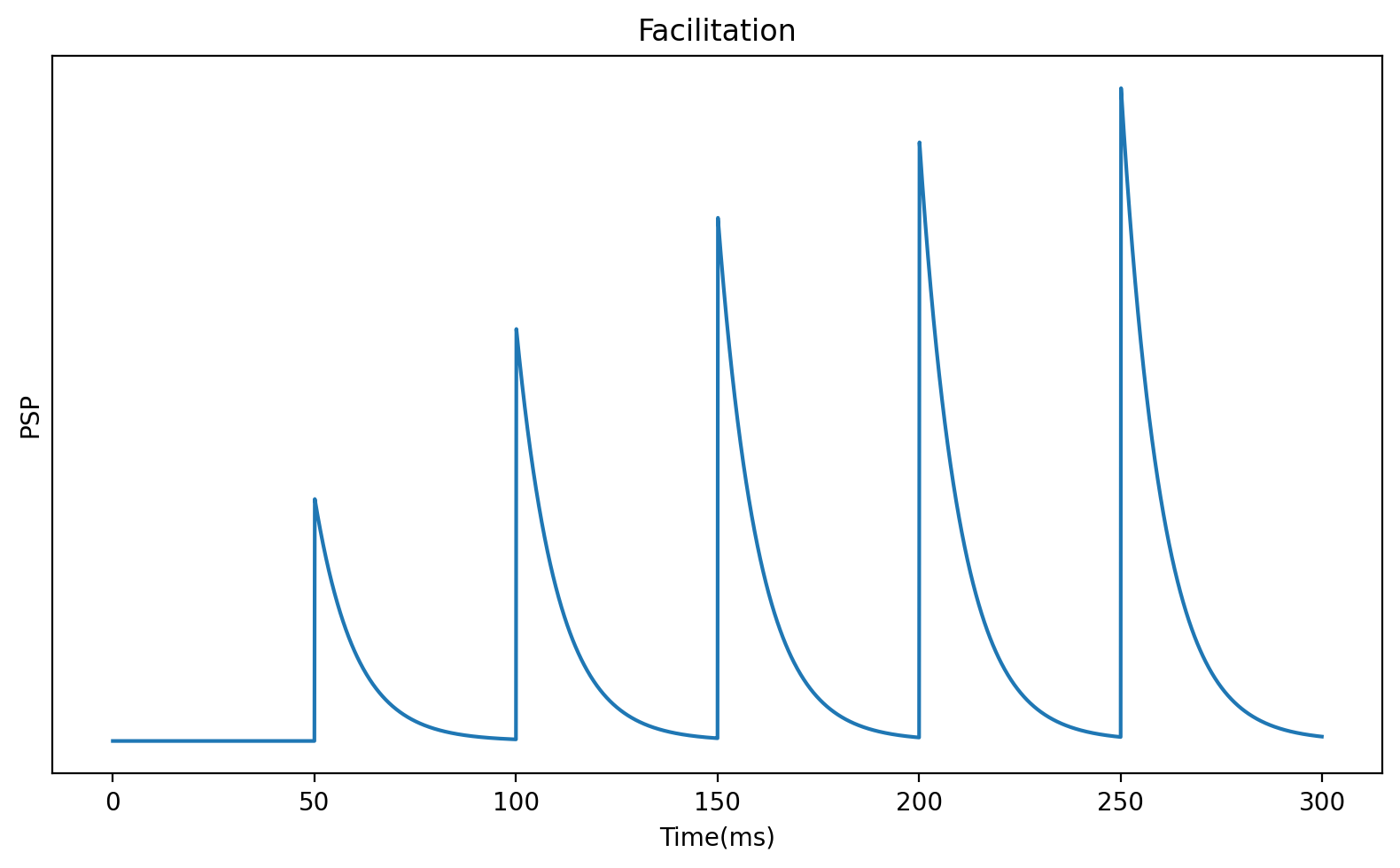
A simple model that encapsulates both effects is to add an extra variable, $u$ , that represents the probability that an available vesicle will be released, and allow this to increase after each spike.

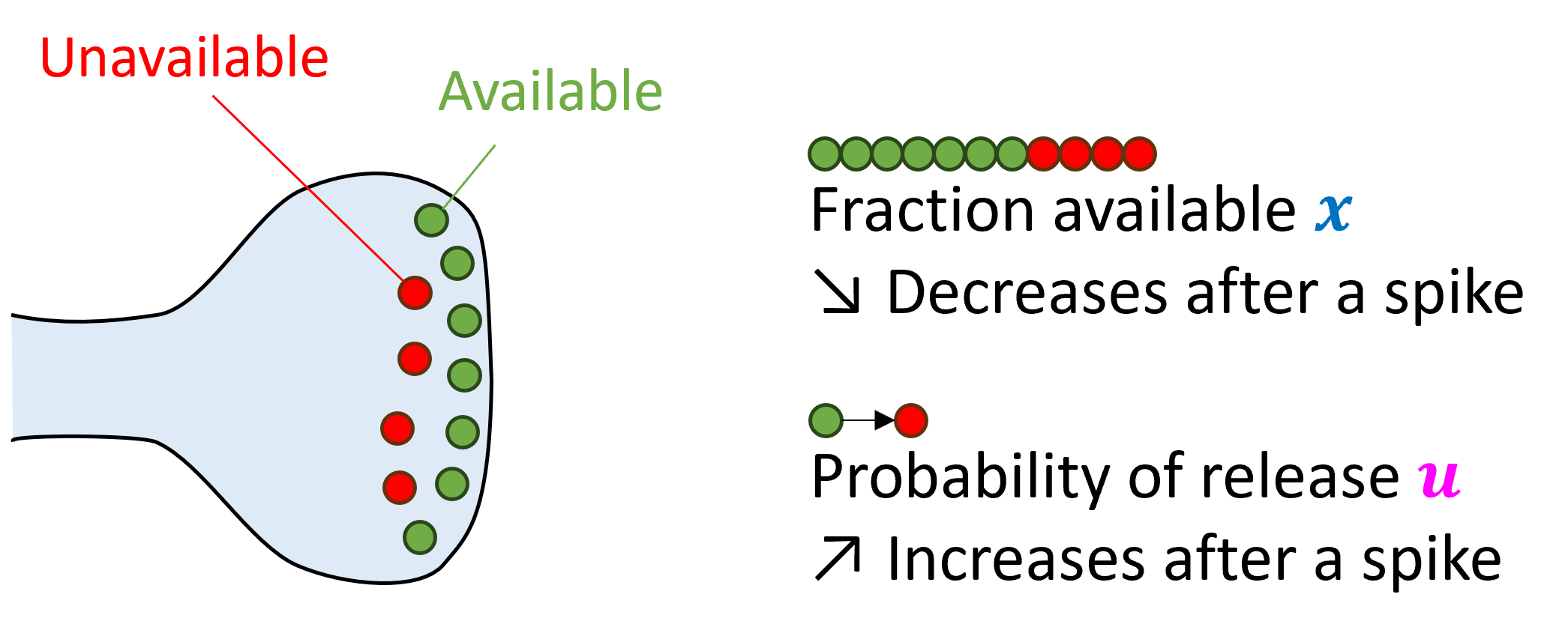
Combining these two ideas in the simplest way possible, we get this model:

Definition of short term plasticity model

At each synapse, we have the following dynamic variables:

$x$ is the fraction of available neurotransmitter, and starts at 1.
$u$ is the probability that a neurotransmitter is released, and starts at 0.

And constants:

$\tau_d$ the decay rate of $x$ that controls the time scale of depression
$\tau_f$ the decay rate of $u$ that controls the time scale of facilitation
$U$ the effect of a spike on $u$ , controlling the scale of facilitation
$A$ is a synaptic weight, controlling the strength of the synapse

In the absence of a spike, the variables evolve continuously following these equations:

\begin{aligned} \tau_f \textcolor{#fc05db}{u}' &= -\textcolor{#fc05db}{u} \\ \tau_d \textcolor{#0a62a6}{x}' &= 1-\textcolor{#0a62a6}{x}\\ \end{aligned}

(13)

When a spike arrives, the following instantaneous changes are made (where $v$ is the post-synaptic potential):

\begin{aligned} \textcolor{#fc05db}{u} &\leftarrow \textcolor{#fc05db}{u} + U \cdot (1-\textcolor{#fc05db}{u}) \\ v &\leftarrow v + A \cdot \textcolor{#fc05db}{u} \cdot \textcolor{#0a62a6}{x} \\ \textcolor{#0a62a6}{x} &\leftarrow \textcolor{#0a62a6}{x} - \textcolor{#fc05db}{u} \cdot \textcolor{#0a62a6}{x} \end{aligned}

(14)

Note that the order of operations matters! If $u=0$ and $x=1$ before the spike, after the first operation $u$ will increase to $U$ , then the post-synaptic potential will then increase by the non-zero quantity $AU$ , and finally $x$ will decrease to $1-U$ .

In the absence of any spikes, the pool of available vesicles will increase exponentially until all vesicles are available.

At the same time, the probability of spiking will decay to 0.

We can control the rate of these processes with facilitation and depression time constants $\tau_f$ and $\tau_d$ .

When a spike arrives, we first increase $u$ , the probability of vesicle release. Note that we do this first because otherwise the first spike would release 0 vesicles.

Next, we release an amount of vesicles proportional to $u \cdot x$ , because there are $x$ available and we release with probability $u$ . In this model we’ve had this directly modify the membrane potential $v$ , but it could modify other variables.

Finally, since we’ve released $u \cdot x$ vesicles, we now have to remove those from the available pool by subtracting that from $x$ .

Here’s what those variables look like in these two cases:

Source:

💻 Code for figures

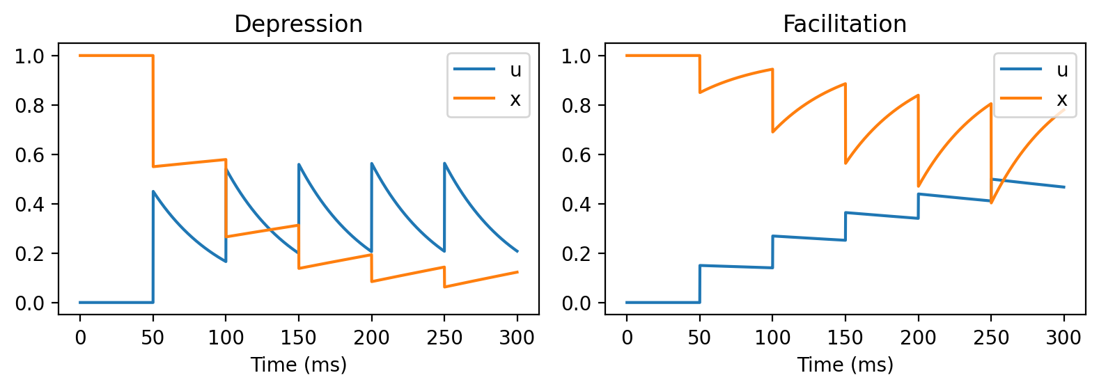
So what does this do in terms of function?

As usual, we don’t have a complete answer to that. One thing for sure is that it gives synapses a longer memory than they would otherwise have, which is likely to be useful in many cases.

It can also allow the neuron to have richer spike frequency dynamics, allowing them to act as low, high or band pass filters, and do gain control. There’s a bunch of other ideas people have suggested, and there are links in the reading list for where you can read more about this and other models of short term plasticity.

Channel types: excitation and inhibition¶

As previously mentioned, synapses can be either excitatory or inhibitory. There are a range of different ion channels and dynamics giving rise to different sorts of excitatory or inhibitory synapses. Channel types include inhibitory ( $GABA_A$ fast and $GABA_B$ slow) and excitatory (AMPA fast and NMDA slow) The simplest model is that excitatory synapses lead to an increase in some variable, while inhibitory synapses lead to a decrease.

Excitation: $v \leftarrow v + w$
Inhibition: $v \leftarrow v - w$

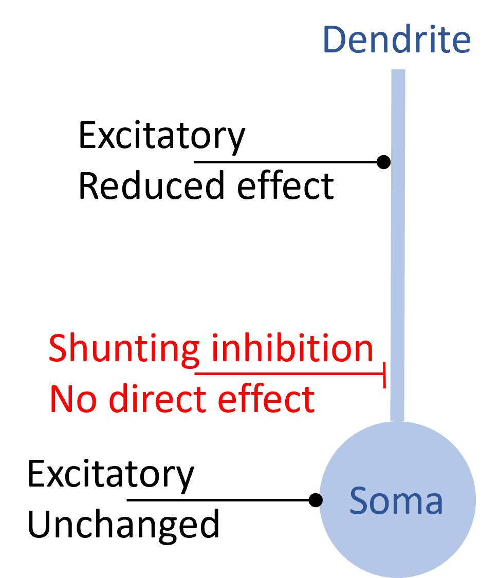
However, when synapses are modelled with detail ion channel dynamics and spatial structure, things can get more interesting. Shunting inhibition is a good example.

In shunting inhibition, a spike causes a local increase in conductance but with a reversal potential near to the resting potential. This means that on its own in the absence of other inputs, you wouldn’t observe any effect on the membrane potential. However, it will reduce the effect of an excitatory synapse on the dendrite while having no effect on an excitatory synapse on the soma or on a different dendritic branch. This means that it can have a selective, divisive effect on excitatory inputs, something you wouldn’t easily be able to achieve otherwise.

Another interesting channel type is NMDA, which can’t be modelled linearly. The effect of NMDA requires the receiving neuron’s membrane potential to have recently been high. This may be important in learning.

Long-term plasticity¶

Talking of learning, we’ll briefly mention long-term plasticity, since this is the main topic of week 4. Earlier, we mentioned the Hebbian rules, and you can generally model them by adding some differential equations for the synaptic weight $w$ as a function of the activity of the pre-synaptic and post-synaptic neurons. We’ll talk about some particular models later.

\frac{\ud w}{\ud t} = \text{ some function of $w$ and pre- and post-synaptic activity}

(15)

Spike timing-dependent plasticity (STDP)¶

It has been observed experimentally that particular pairings of pre- and post-synaptic spike times can lead synapses to get stronger or weaker. We can model this by increasing the weight by some $\Delta w$ that depends on the timing difference, which can be made a reasonable fit to experimental data. This particular curve, where the synapse gets stronger if pre-synaptic spikes tend to come before post-synaptic spikes, could be thought of as encouraging networks to care about temporal causality. We will cover this in more detail later on.

\Delta w = \sum_{\substack{\text{pre-synaptic}\\\text{spikes }t_j}} \;\; \sum_{\substack{\text{post-synaptic}\\\text{spikes }t_i}} W(t_i - t_j)

(16)

where

W(\delta t) = \begin{cases} A_+ e^{-\frac{\delta t}{\tau_+}} \quad \text{for } \delta t > 0 \\ A_- e^{-\frac{\delta t}{\tau_-}} \quad \text{for } \delta t < 0 \end{cases}

(17)

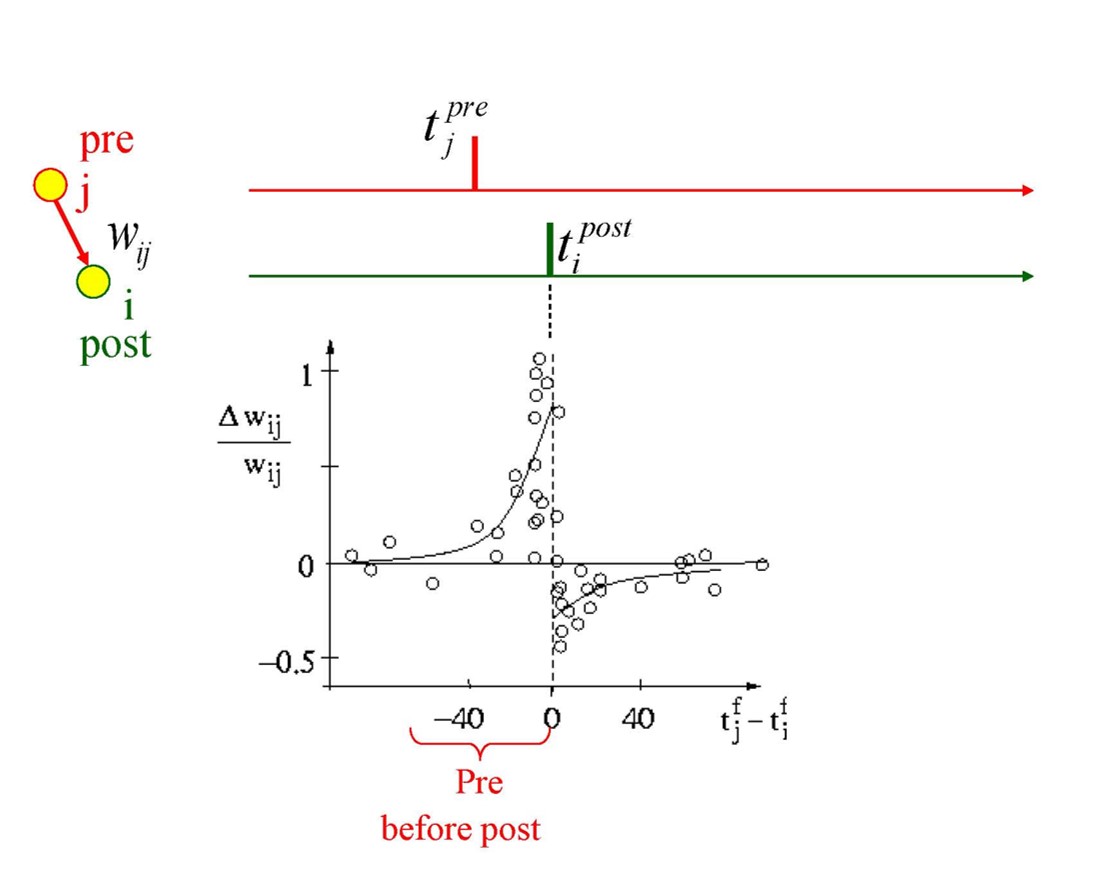
Figure 5:Synapse behavior with pre and post-synaptic spikes

More synaptic fun¶

As always, there’s a lot more that could be said about modelling synapses. We’ll just briefly mention 2. The first is synaptic failure. It’s easy to model by adding a chance of failure to each synaptic event.

v \leftarrow v + w \text{ (with probability $p$)}

(18)

The second is gap junctions - when two neurons form a direct electrical connection rather than a chemical synapse. These can again be straight forwardly modelled as just another current proportional to the difference in membrane potentials. There are of course more complicated models too.

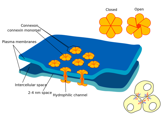
\begin{aligned} \tau v' &= I_\text{gap} - v \\ I_\text{gap} &= w(v_\text{pre} - v_\text{post}) \end{aligned}

(19)

Gap junctions occur in many species, but a particularly interesting example is the tiny worm caenorhabditis elegans (usually written C. elegans). Neuroscientists love it because it always has precisely 302 neurons with the same pattern of connections. It’s unusual though because they are mostly non-spiking, using gap junctions to communicate instead.

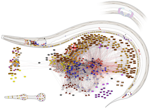
C. elegans connectome. — Figure 7:*C. elegans* connectome.

Week 2 - Synapses and networks

Networks

Week 2 - Synapses and networks

Network models