Introduction
In the first week we’re going to focus on neurons - which are thought to be the brain’s primary processing units. We’ll cover 3 topics:
- Neuron structure.
- Neuron function.
- How we can model neurons mathematically and simulate them in code.
Sensorimotor transformation
We can think of both artificial neural networks and brains as computing input-output transformations. That is, they take input data, and output decisions.
For example, a trained ANN may take in images and output classes. Similarly, a predator may use its senses, like vision and hearing, to distinguish prey from other animals. In neuroscience we call this the sensorimotor transformation.
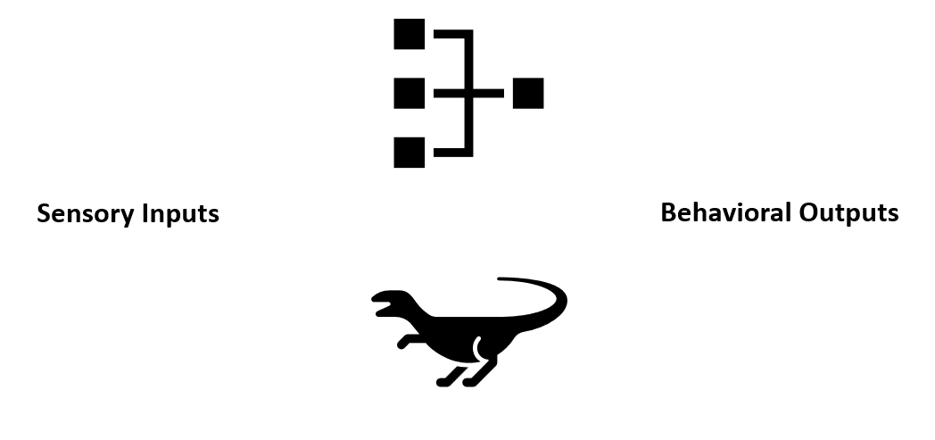
The sensorimotor transformation.
So, how do these systems compute these transformations?
Units and neurons
In ANNs, these transformations are realized by units - which sum their weighted inputs and pass them through an activation function (like ReLU).
In brains, the equivalent are neurons which are not just simple points, but complex 3D structures, like the neuron shown here. Just to give you an idea of scale, the human brain contains around 86 billion neurons.

Figure 2:An artificial unit (left) versus a real neuron (right).
So, what makes up a neuron?
Neurons
Like other cells, neurons have:
- A fatty membrane which separates their inner contents from their surroundings.
- Then inside, they are filled with a fluid known as cytoplasm.
- In their cytoplasam, you’ll find things which are found in other cells, like a nucleus containing genetic material, which sits in their main cell body or soma.
But, unlike many other cells, neurons act as information processing units:
- Neurons receive inputs from other neurons via their dendritic tree. Shown on the left.
- Then they signal to other neurons, muscles or glands, via their axon. Shown on the right.
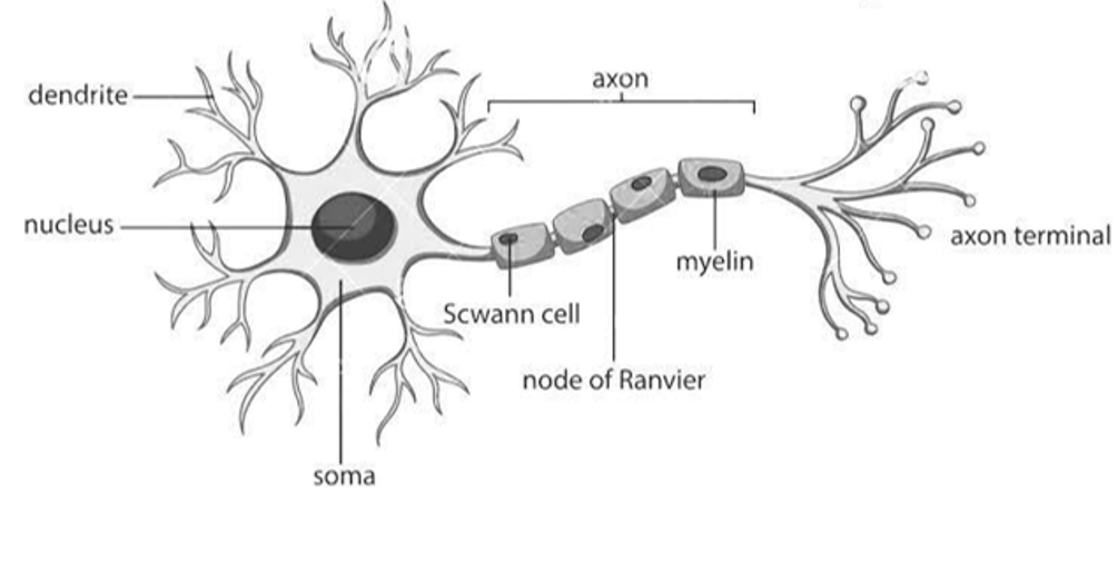
Figure 3:Diagram of a neuron.
For example, Scala et al. (2020) made detailed measurements from over 1,000 neurons and concluded that there were around 70 types: which differ in several features - including their morphology, which you can see here. Some of the neurons in blue look like the diagram we saw on the previous slide, but others, like those in pink look quite different.
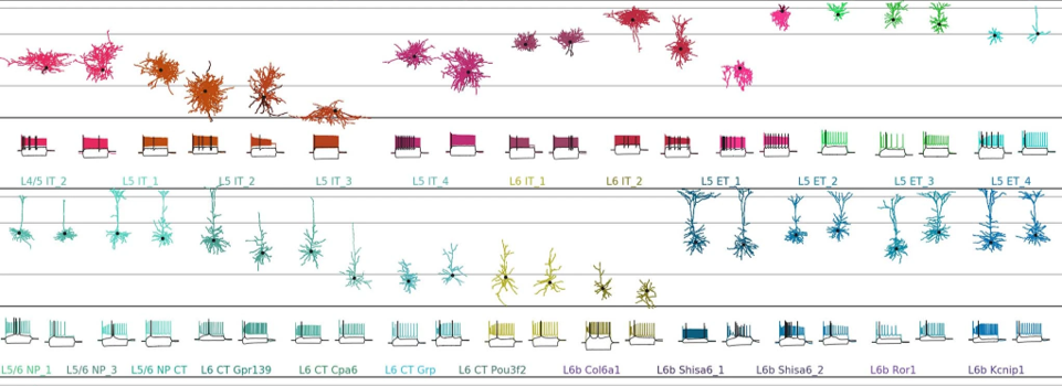
Figure 4:The diversity of neuron morphologies. From Scala et al. (2020).
While you might assume that this complexity was reserved for, or unique to, the human brain.
All of these 70 neuron types, and actually this whole study, is focused on just one part of the mouse brain.
So, is this structural diversity just random, i.e. the result of noisy biological processes, or not?
Is neural structure random?
Chandrasekhar & Navlakha (2019) analysed the morphology of over 10,000 real neurons from an open source dataset and show that they balance wiring costs and conduction delays.
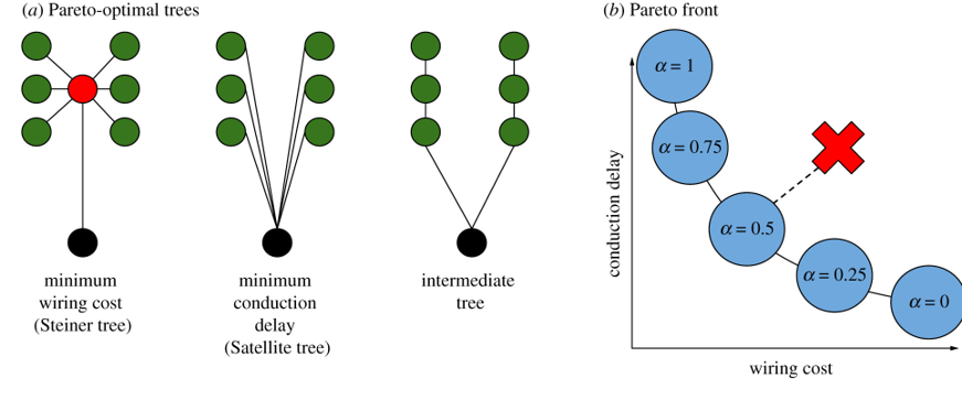
Figure 5:Analysis of neuron morphology Chandrasekhar & Navlakha, 2019.
In Figure 5a, the black circles represent the soma or cell body of the neuron. The green circles, show the inputs, and the red circle shows a branch point. And what this figure shows is how it’s possible to wire the connections from green to black in different ways.
On the left, is the tree with the minimum wiring cost. In the middle is the tree with the minimum conduction delay. On the right is an intermediate tree.
Now, as these two objectives, minimizing wiring cost and conduction delay, compete with each other, they form a Pareto front, where improving one leads to a loss in the other. This is shown in Figure 5b, where the x axis is the wiring cost, the y-axis is the conduction delay, and the front shows how improving one impairs the other. For example, decreasing the conduction delay leads to an increase in wiring cost.
Then with this front defined, you can measure how far any given tree falls from it, as shown by the red cross.
What the authors conclude is:
- That neural arbors are much closer to being Pareto optimal than you would expect by chance.
- Suggesting that neuron structure is not random, but strikes a balance between optimizing wiring cost and conduction delays.
So, how does this sort of structure impact computation?
How does structure impact computation?
Frankly, that’s an open question, so rather than giving you an answer, we’re just going to give you one example of the type of work people are pursuing in this direction.
Jones & Kording (2021) model a single neuron and study how changing the properties of it’s dendritic tree (which process it’s inputs) alters it’s ability to solve classic machine learning benchmarks like MNIST.
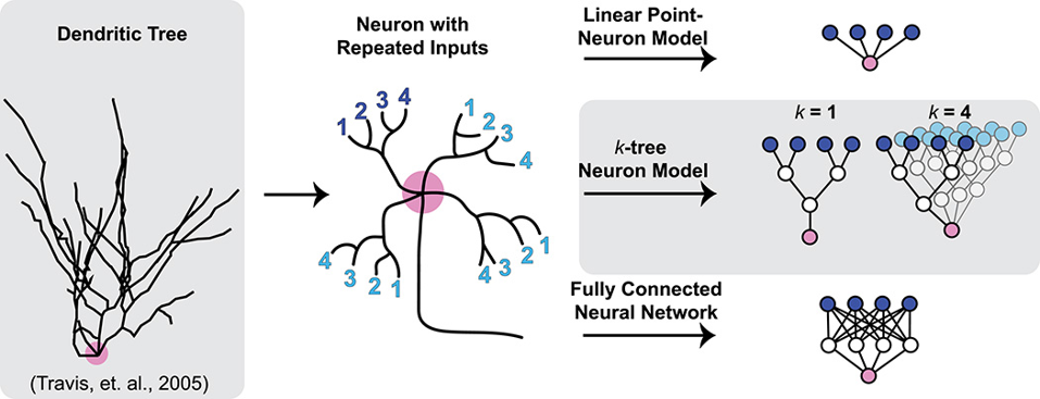
Figure 6:Modelling dendritic trees with artificial neural networks Jones & Kording, 2021.
Shown on the left here is an outline of a real neuron. It’s cell body is marked in pink and the black lines show it’s dendritic tree. From examining these trees, researchers have found two interesting features: their branched morphology and repeated inputs.
These features are shown schematically in the middle. Here we have a single neuron with it’s soma in pink, an output axon, and four numbered inputs, in dark blue, to it’s dendritic tree. As you can see these inputs are divided into two branches, and this structure is repeated across sub-trees which are shown in light blue.
So, in this paper, the authors study how altering the structure of this tree, which they call a k-tree neuron model, impacts task performance. As a lower bound, they use a linear point neuron model, and as an upper bound they use a fully connected neural network with the same number of trainable parameters.
What they conclude is that:
- The performance of their tree model improves as you increase k (the number of repeated subtrees).
- But degrades when you make the trees more realistic by making them asymmetrical.
Which suggests that there is still lots left to explore in this space!
- Scala, F., Kobak, D., Bernabucci, M., Bernaerts, Y., Cadwell, C. R., Castro, J. R., Hartmanis, L., Jiang, X., Laturnus, S., Miranda, E., Mulherkar, S., Tan, Z. H., Yao, Z., Zeng, H., Sandberg, R., Berens, P., & Tolias, A. S. (2020). Phenotypic variation of transcriptomic cell types in mouse motor cortex. Nature, 598(7879), 144–150. 10.1038/s41586-020-2907-3
- Chandrasekhar, A., & Navlakha, S. (2019). Neural arbors are Pareto optimal. Proceedings of the Royal Society B: Biological Sciences, 286(1902), 20182727. 10.1098/rspb.2018.2727
- Jones, I. S., & Kording, K. P. (2021). Might a Single Neuron Solve Interesting Machine Learning Problems Through Successive Computations on Its Dendritic Tree? Neural Computation, 33(6), 1554–1571. 10.1162/neco_a_01390