Introduction
So far this week we’ve seen a lot of biological detail about neurons. The topic of this section is how we abstract and simplify this into very simple models.
Artificial neuron
You’re probably familiar with the artificial neuron from machine learning.
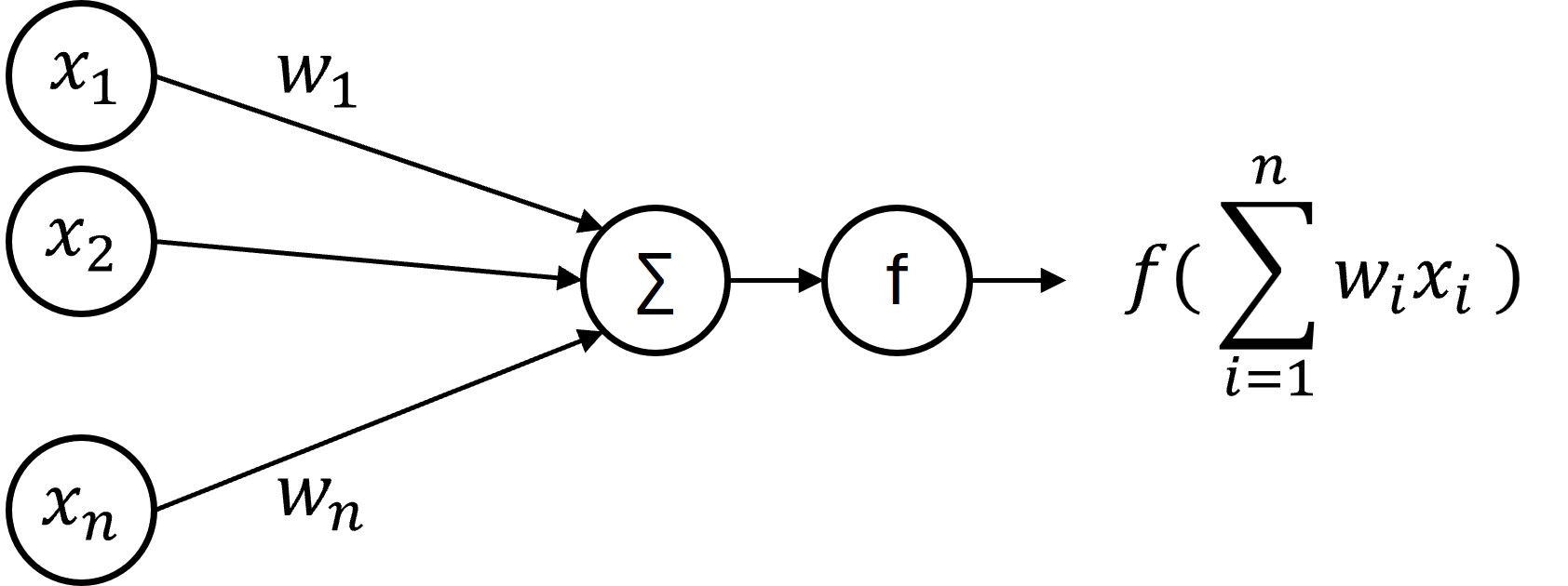
Figure 1:Single artificial neuron.
This neuron has inputs, which have activations to with weights to . Each of these activations and weights is a real number.
It performs a weighted sum of its inputs and then passes that through some nonlinear function :
Various activation functions can be used here. In older work you’ll often see the sigmoid function, and that’s partly because it was considered a good model of real neurons. Nowadays, you’ll more often see the ReLU, which turns out to be much easier to work with and gives results that are often better.

Figure 2:Common activation functions for an artificial neuron.
Interestingly, there are papers still being published about what the best model of real neurons’ activation functions, like LaFosse et al. (2023) which finds an activation function that looks a bit intermediate between sigmoid and ReLU.
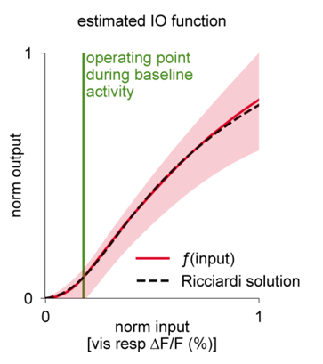
Figure 3:Estimated activation function from real neurons (from LaFosse et al. (2023)).
The relationship between the model and the biological data is established by computing an input-output function, typically by counting the number of spikes coming in to the neurons versus the number of spikes going out, averaged over multiple runs and some time period.
What this model misses out is the temporal dynamics of biological neurons.
Biological neuron
So let’s talk about temporal dynamics. We saw in previous sections that when a neuron receives enough input current it pushes it above a threshold that leads to an action potential, also called a spike.
The source of the input current is incoming spikes from other neurons, and we’ll talk more about that in next week’s sections on synapses.
For this week, here’s a simple, idealised picture of what this looks like. It’s from a model rather than real data, to more clearly illustrate the process.
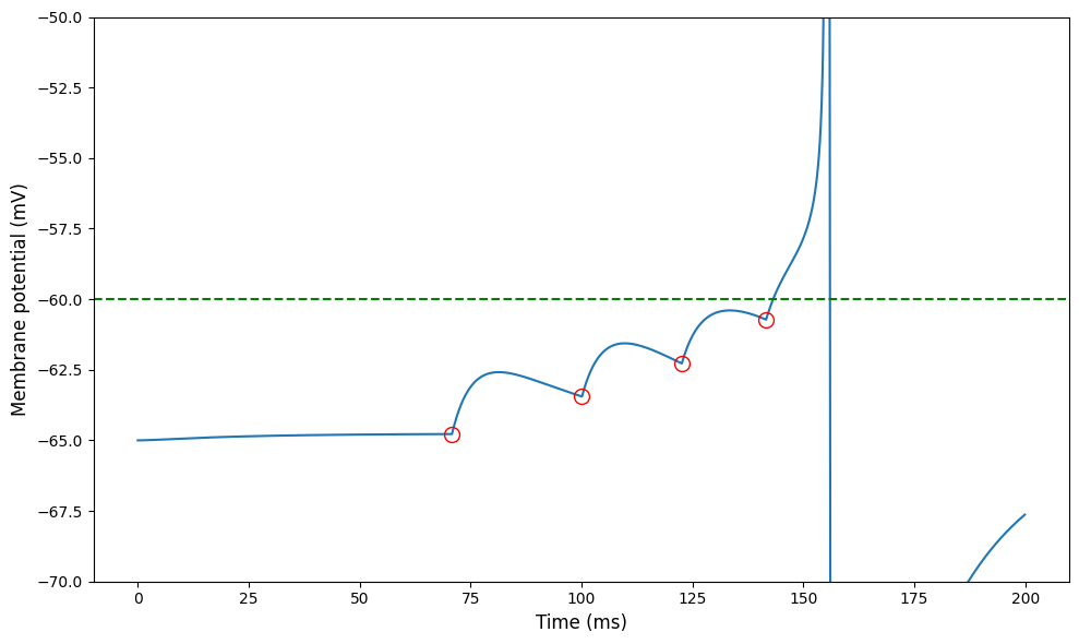
The curve shows the membrane potential of a neuron receiving input spikes at the times indicated by the red circles. Each incoming spike causes a transient rush of incoming current.
For the first one, it’s not enough to cause the neuron to spike, and after a while the membrane potential starts to decay back to its resting value.
And then, more come in and eventually the cumulative effect is enough to push the neuron above the threshold, and it fires a spike and resets.
Integrate and Fire Neuron
The simplest way to model this is using the “integrate and fire neuron”. Here’s a plot of how it behaves.
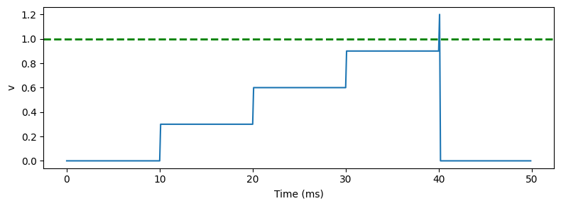
Each time an incoming spike arrives - every 10 milliseconds here - the membrane potential instantaneously jumps by some fixed weight until it hits the threshold, at which point it fires a spike and resets.
We can write this down in a standard form as a series of event-based equations.
- When you receive an incoming spike, set the variable to be .
- If the threshold condition () is true, fire a spike.
- After a spike, set to 0.
Table 1:Integrate and fire neuron definition
| Condition | Model behaviour |
|---|---|
| On presynaptic spike index | |
| Threshold condition, fire a spike if | |
| Reset event, after a spike set |
We can see that already this captures part of what’s going on in a real neuron, but misses the fact that in the absence of new inputs, the membrane potential decays back to rest. Let’s add that.
Leaky integrate-and-fire (LIF) neuron
We can model this decay by treating the membrane as a capacitor in an electrical circuit. Turning this into a differential equation, evolves over time according to the differential equation:
where τ is the membrane time constant discussed earlier. We can summarise this as a table as before:
Table 2:Leaky integrate-and-fire neuron definition
| Condition | Model behaviour |
|---|---|
| Continuous evolution over time | |
| On presynaptic spike index | |
| Threshold condition, fire a spike if | |
| Reset event, after a spike set |
This differential equation can be solved to show that in the absence of any input, decreases exponentially over time with a time scale of τ:
Here’s how that looks:
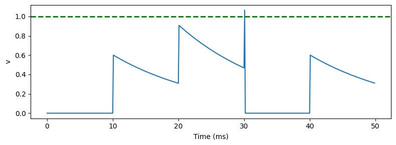
We can see that after the instantaneous increase in membrane potential it starts to decay back to the resting value. Although this doesn’t look like a great model, it turns out that very often this captures enough of what is going on in real neurons.
But there is another reason why adding this leak might be important.
Reliable spike timing
In experiments, if you inject a constant input current (horizontal line, top left) into a neuron and record what happens over a few repeated trials, you see that the membrane potentials (top left above input current) and the spike times (bottom left) are fairly different between trials. That’s because there’s a lot of noise in the brain which adds up over time.
On the other hand, if you inject a fluctuating input current (top right) and do the same thing, you’ll see both the membrane potentials (top right, above fluctuating current) and the spikes (bottom right) tend to occur at the same times. The vertical lines on the bottom right plot show that on every repeat, the spike is happening at the same time.
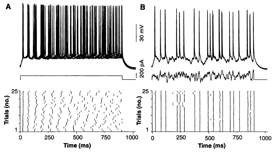
Figure 4:Raster plots for constant and fluctuating input current Mainen & Sejnowski, 1995.
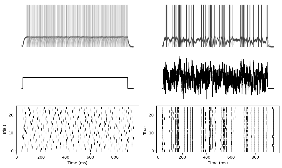
We see the same thing with a LIF neuron. Here are the plots with semi-transparent membrane potentials so that you can clearly see that both the spike times and membrane potentials tend to overlap for the fluctuating current, but not the constant current.
But now if we repeat that with a simple integrate and fire neuron without a leak, you can see you get unreliable, random spike times for both the constant and fluctuating currents.
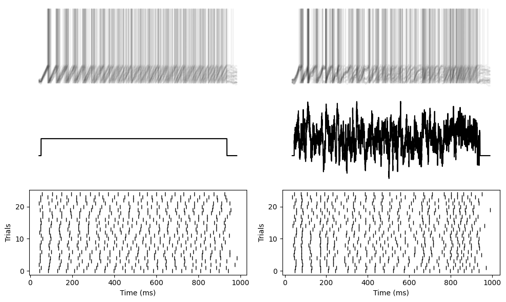
In other words, adding the leak made the neuron more robust to noise. An important property for the brain, and perhaps also for low power neuromorphic hardware that we’ll talk about later in the course.
So why does the leak make it more noise robust? Well that was answered by Brette & Guigon (2003). The mathematical analysis is complicated, but it boils down to the fact that if you either have a leak, or a nonlinearity in the differential equations, the fluctuations due to the internal noise don’t accumulate over time, whereas with a linear and non-leaky neuron, they do.
LIF neuron with synapses
OK, so we have an LIF neuron which we’ve just seen has some nice properties that you’d want a biological neuron model to have. But still, when you look at the graph here, you can see that these instantaneous jumps in the model are not very realistic. So how can we improve that?
A simple answer is to change the model so that instead of having an instantaneous effect on the membrane potential, instead it has an instantaneous effect on an input current, which is then provided as an input to the leaky integrate-and-fire neuron.
You can see on the bottom plot here that the input current is now behaving like the membrane potential before, with this exponential shape. You can think of that as a model of the internal processes of the synapses that we’ll talk more about next week.
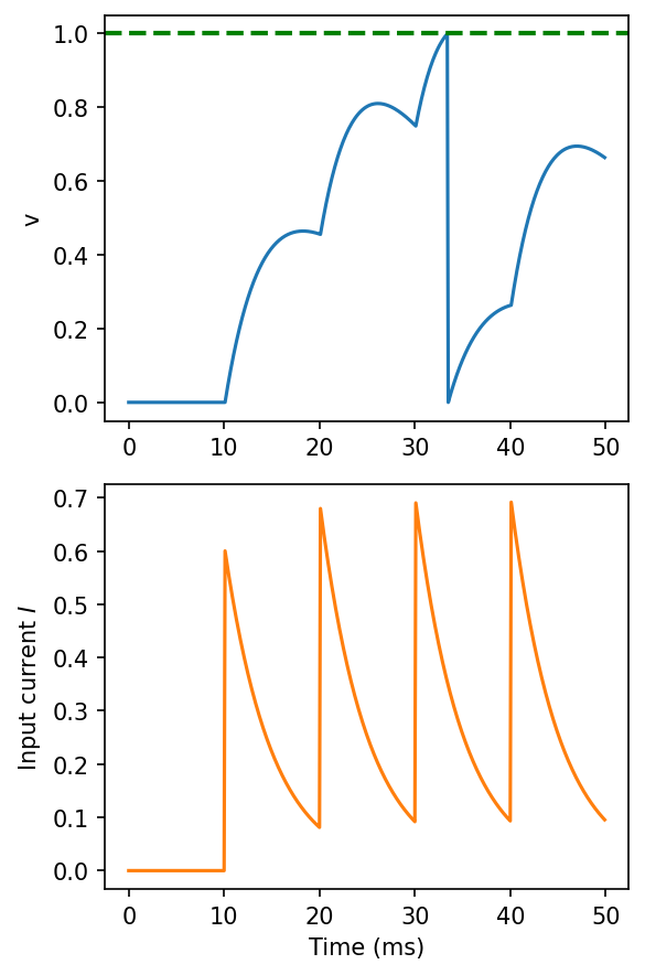
Figure 5:Leaky integrate-and-fire with exponential synapses.
We model that by adding a differential equation, with its own time constant :
We also add that current to the differential equation for , multiplied by a constant . The rest of the model is as it was before:
Table 3:Leaky integrate-and-fire neuron with exponential synapses definition
| Condition | Model behaviour |
|---|---|
Continuous evolution over time | |
| On presynaptic spike index | |
| Threshold condition, fire a spike if | |
| Reset event, after a spike set |
We can see that this gives a better approximation of the shape. There’s more that can be done here if you want, for example modelling changes in conductance rather than current, but we’ll get back to that next week.
Spike frequency adaptation
If you feed a regular series of spikes into an LIF neuron (without any noise) you’ll see that the time between spikes is always the same. It has to be because the differential equation is memoryless and resets after each spike.
However, real neurons have a memory of their recent activity. Here are some recordings from the Allen Institute cell types database that we’ll be coming back to later in the course.
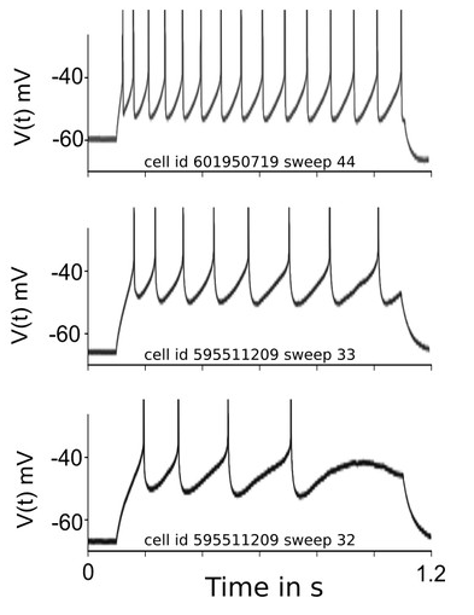
Figure 6:Example of spike frequency adaptation Salaj et al., 2021.
In these recordings (from Salaj et al. (2021)), they’ve injected a constant current into these three different neurons, and recorded their activity. We can see that rather than outputting a regularly spaced sequence of spikes, there’s an increasing gap between the spikes. There are various mechanisms underlying this, but essentially it comes down to slower processes that aren’t reset by a spike. Let’s see how we can model that.
Actually there are many, many different models for spike frequency adaptation. We’ll just show one very simple approach, but if you want some more ideas it’s reviewed in Gutkin & Zeldenrust (2014).
In the simple model here, we just introduce a variable threshold represented by the variable . Each time the neuron spikes, the threshold increases, making it more difficult to fire the next spike, before slowly decaying back to its starting value.
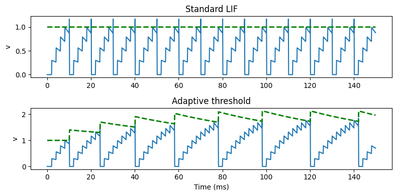
Figure 7:Spike frequency adaptation model compared to standard LIF.
In the equations, we represent that by having a new exponentially decaying differential equation for the threshold, modifying the threshold condition so that it’s instead of , and specifying that after a spike the threshold should increase by some value. You can see that it does the job, there’s a smaller gap between earlier spikes than later spikes.
Table 4:Adaptive leaky integrate-and-fire neuron definition
| Condition | Model behaviour |
|---|---|
Continuous evolution over time | |
| On presynaptic spike index | |
| Threshold condition, fire a spike if | |
Reset event, after a spike set |
In general, spike frequency adaptation can give really rich and powerful dynamics to neurons, but we won’t go into any more detail about that right now.
Other abstract neuron models
This has been a quick tour of some features of abstract neuron models. There’s a lot more to know about if you want to dive deeper.
Some of the behaviours of real neurons that we haven’t seen in our models so far include:
- Phasic spiking, i.e. only spiking at the start of an input.
- Bursting, both phasic at the start or tonic ongoing.
- And post-inhibitory rebound, where a neuron fires a spike once an inhibitory or negative current is turned off.
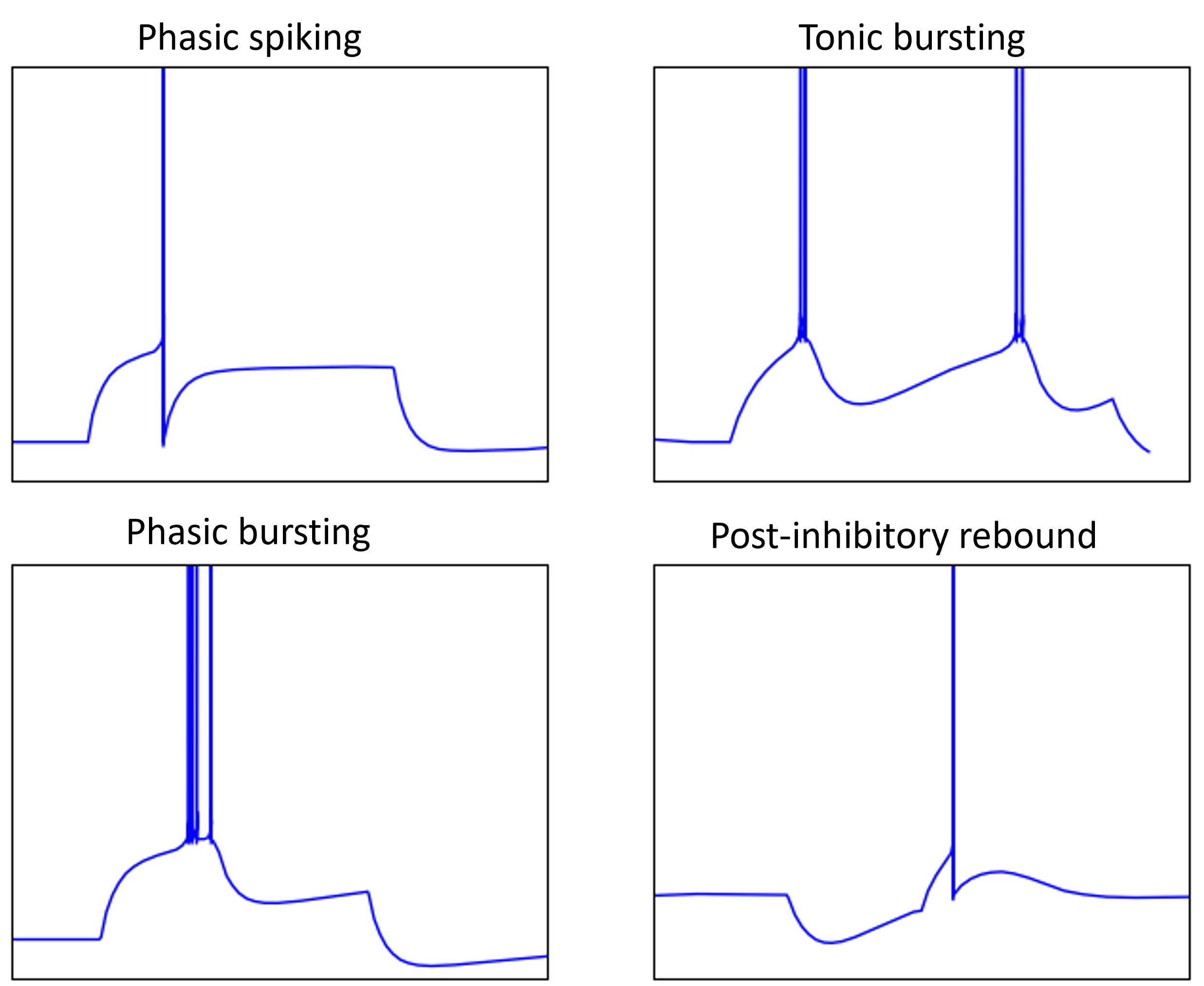
Figure 8:Behaviours of real neurons.
You can capture a lot of these effects with two variable models such as the adaptive exponential integrate and fire or Izhikevich neuron models.
There’s also stochastic neuron models based either on having a Gaussian noise current or a probabilistic spiking process.
Taking that further there are Markov chain models of neurons where you model the probability of neurons switching between discrete states.
For more
You can find the code to generate the figures from this section in 💻 Code for figures.
Further reading:
- LaFosse, P. K., Zhou, Z., O’Rawe, J. F., Friedman, N. G., Scott, V. M., Deng, Y., & Histed, M. H. (2023). Single-cell optogenetics reveals attenuation-by-suppression in visual cortical neurons. 10.1101/2023.09.13.557650
- Mainen, Z. F., & Sejnowski, T. J. (1995). Reliability of Spike Timing in Neocortical Neurons. Science, 268(5216), 1503–1506. 10.1126/science.7770778
- Brette, R., & Guigon, E. (2003). Reliability of Spike Timing Is a General Property of Spiking Model Neurons. Neural Computation, 15(2), 279–308. 10.1162/089976603762552924
- Salaj, D., Subramoney, A., Kraisnikovic, C., Bellec, G., Legenstein, R., & Maass, W. (2021). Spike frequency adaptation supports network computations on temporally dispersed information. eLife, 10. 10.7554/elife.65459
- Gutkin, B., & Zeldenrust, F. (2014). Spike frequency adaptation. Scholarpedia, 9(2), 30643. 10.4249/scholarpedia.30643