The code below generates the figures used in the notebooks, and might be useful to explore these ideas further.
Neuron models
It makes use of the Brian spiking neural network simulator package. Feel free to have a play with this and explore its documentation, including excellent tutorials.
!pip install brian2
import os
from brian2 import *
prefs.codegen.target = 'numpy'“Biological” neurons
This is just a Hodgkin-Huxley neuron modified to include exponential current synapses (as we do later for the integrate-and-fire neuron).
start_scope()

duration = 200*ms

# Parameters
area = 20000*umetre**2
Cm = (1*ufarad*cm**-2) * area
gl = (5e-5*siemens*cm**-2) * area

El = -65*mV
EK = -90*mV
ENa = 50*mV
g_na = (100*msiemens*cm**-2) * area
g_kd = (30*msiemens*cm**-2) * area
VT = -63*mV
# Time constants
taue = 5*ms
taui = 10*ms
# Reversal potentials
Ee = 0*mV
Ei = -80*mV
we = 2*nS  # excitatory synaptic weight
wi = 67*nS  # inhibitory synaptic weight

# The model
eqs = Equations('''
dv/dt = (gl*(El-v)+ge*(Ee-v)+gi*(Ei-v)-
         g_na*(m*m*m)*h*(v-ENa)-
         g_kd*(n*n*n*n)*(v-EK))/Cm : volt
dm/dt = alpha_m*(1-m)-beta_m*m : 1
dn/dt = alpha_n*(1-n)-beta_n*n : 1
dh/dt = alpha_h*(1-h)-beta_h*h : 1
dge/dt = -ge*(1./taue) : siemens
dgi/dt = -gi*(1./taui) : siemens
alpha_m = 0.32*(mV**-1)*4*mV/exprel((13*mV-v+VT)/(4*mV))/ms : Hz
beta_m = 0.28*(mV**-1)*5*mV/exprel((v-VT-40*mV)/(5*mV))/ms : Hz
alpha_h = 0.128*exp((17*mV-v+VT)/(18*mV))/ms : Hz
beta_h = 4./(1+exp((40*mV-v+VT)/(5*mV)))/ms : Hz
alpha_n = 0.032*(mV**-1)*5*mV/exprel((15*mV-v+VT)/(5*mV))/ms : Hz
beta_n = .5*exp((10*mV-v+VT)/(40*mV))/ms : Hz
''')
# Threshold and refractoriness are only used for spike counting
group = NeuronGroup(1, eqs, threshold='v>-20*mV', refractory=3*ms,
                method='exponential_euler')
group.v = El

# Little trick to get a sequence of input spikes that get faster and faster
inp_sp = NeuronGroup(1, 'dv/dt=int(t<150*ms)*t/(50*ms)**2:1', threshold='v>1', reset='v=0', method='euler')
S = Synapses(inp_sp, group, on_pre='ge += we')
S.connect(p=1)

monitor = StateMonitor(group, 'v', record=True)
input_monitor = SpikeMonitor(inp_sp)

run(duration)

figure(figsize=(10,6))
plot(monitor.t/ms, monitor.v[0]/mV)
ylim(-70, -50)
ylabel('Membrane potential (mV)', fontsize=12)
xlabel('Time (ms)', fontsize=12)
tight_layout()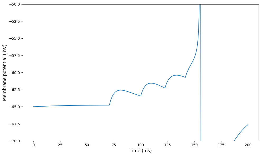
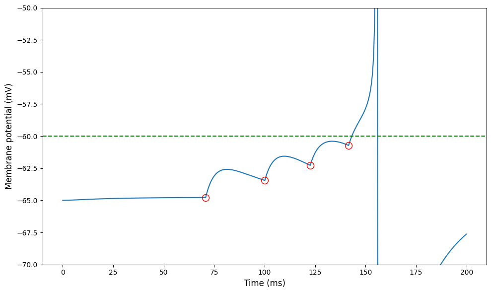
Version for website
figure(figsize=(10,6))
plot(monitor.t/ms, monitor.v[0]/mV)
plot(input_monitor.t/ms, monitor.v[0][array(input_monitor.t/inp_sp.dt, dtype=int)]/mV, 'o', color='r', mfc='none', ms=10)
axhline(-60, ls='--', color='g')

ylim(-70, -50)
ylabel('Membrane potential (mV)', fontsize=12)
xlabel('Time (ms)', fontsize=12)
tight_layout();
Integrate and fire neuron
start_scope()

duration = 50*ms

eqs = '''
dv/dt = 0/second : 1
'''
G_out = NeuronGroup(1, eqs, threshold='v>1', reset='v=0', method='euler')
nspikes_in = 100
timesep_in = 10*ms
G_in = SpikeGeneratorGroup(1, [0]*nspikes_in, (1+arange(nspikes_in))*timesep_in)
S = Synapses(G_in, G_out, on_pre='v += 0.3')
S.connect(p=1)
M = StateMonitor(G_out, 'v', record=True)
run(duration)
figure(figsize=(8, 3))
plot(M.t/ms, M.v[0])
xlabel('Time (ms)')
ylabel('v')
axhline(1, ls='--', c='g', lw=2)
tight_layout()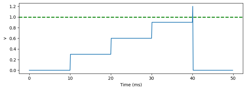
Leaky integrate and fire neuron
start_scope()

duration = 50*ms

eqs = '''
dv/dt = -v/(15*ms) : 1
'''
G_out = NeuronGroup(1, eqs, threshold='v>1', reset='v=0', method='euler')
nspikes_in = 100
timesep_in = 10*ms
G_in = SpikeGeneratorGroup(1, [0]*nspikes_in, (1+arange(nspikes_in))*timesep_in)
S = Synapses(G_in, G_out, on_pre='v += 0.6')
S.connect(p=1)
M = StateMonitor(G_out, 'v', record=True)
run(duration)
figure(figsize=(8, 3))
plot(M.t/ms, M.v[0])
xlabel('Time (ms)')
ylabel('v')
axhline(1, ls='--', c='g', lw=2)
tight_layout()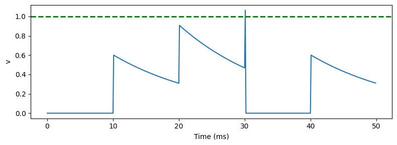
Reliable spike timing
This is the figure we want to reproduce from Mainen and Sejnowski (1995).
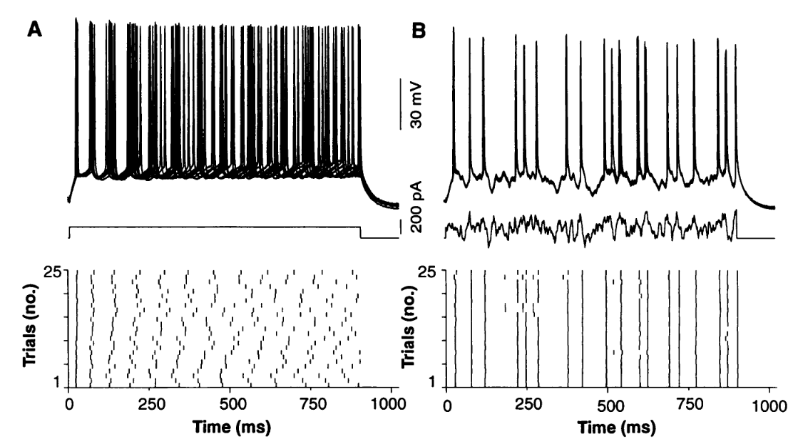
And here’s some Brian code that does the same thing with a leaky integrate and fire neuron.
figure(figsize=(10, 6))

# Neuron equations and parameters
tau = 10*ms
sigma = .03
eqs_neurons = '''
dx/dt = (.65*I - x) / tau + sigma * (2 / tau)**.5 * xi : 1
I = I_shared*int((t>10*ms) and (t<950*ms)) : 1
I_shared : 1 (linked)
'''

start_scope()

# The common input
N = 25
neuron_input = NeuronGroup(1, 'x = 1.5 : 1', method='euler')

# The noisy neurons receiving the same input
neurons = NeuronGroup(N, model=eqs_neurons, threshold='x > 1',
                      reset='x = 0', refractory=5*ms, method='euler')
neurons.x = 'rand()*0.2'
neurons.I_shared = linked_var(neuron_input, 'x') # input.x is continuously fed into neurons.I
spikes = SpikeMonitor(neurons)
M = StateMonitor(neurons, ('x', 'I'), record=True)

run(1000*ms)

def add_spike_peak(x, t, i):
    T = array(rint(t/defaultclock.dt), dtype=int)
    y = x.copy()
    y[T, i] = 4
    return y

ax_top = subplot(321)
plot(M.t/ms, add_spike_peak(M.x[:].T, spikes.t[:], spikes.i[:]), '-k', alpha=0.05)
ax_top.set_frame_on(False)
xticks([])
yticks([])
ax_mid = subplot(323)
plot(M.t/ms, M.I[0], '-k')
ax_mid.set_frame_on(False)
xticks([])
yticks([])
subplot(325)
plot(spikes.t/ms, spikes.i, '|k')
xlabel('Time (ms)')
ylabel('Trials')

start_scope()

# The common noisy input
N = 25
tau_input = 3*ms
neuron_input = NeuronGroup(1, 'dx/dt = (1.5-x) / tau_input + (2 /tau_input)**.5 * xi : 1', method='euler')

# The noisy neurons receiving the same input
neurons = NeuronGroup(N, model=eqs_neurons, threshold='x > 1',
                      reset='x = 0', refractory=5*ms, method='euler')
neurons.x = 'rand()*0.2'
neurons.I_shared = linked_var(neuron_input, 'x') # input.x is continuously fed into neurons.I
spikes = SpikeMonitor(neurons)
M = StateMonitor(neurons, ('x', 'I'), record=True)

run(1000*ms)

ax = subplot(322, sharey=ax_top)
plot(M.t/ms, add_spike_peak(M.x[:].T, spikes.t[:], spikes.i[:]), '-k', alpha=0.05)
ax.set_frame_on(False)
xticks([])
yticks([])
ax = subplot(324, sharey=ax_mid)
plot(M.t/ms, M.I[0], '-k')
ax.set_frame_on(False)
xticks([])
yticks([])
subplot(326)
plot(spikes.t/ms, spikes.i, '|k')
xlabel('Time (ms)')
ylabel('Trials')

tight_layout()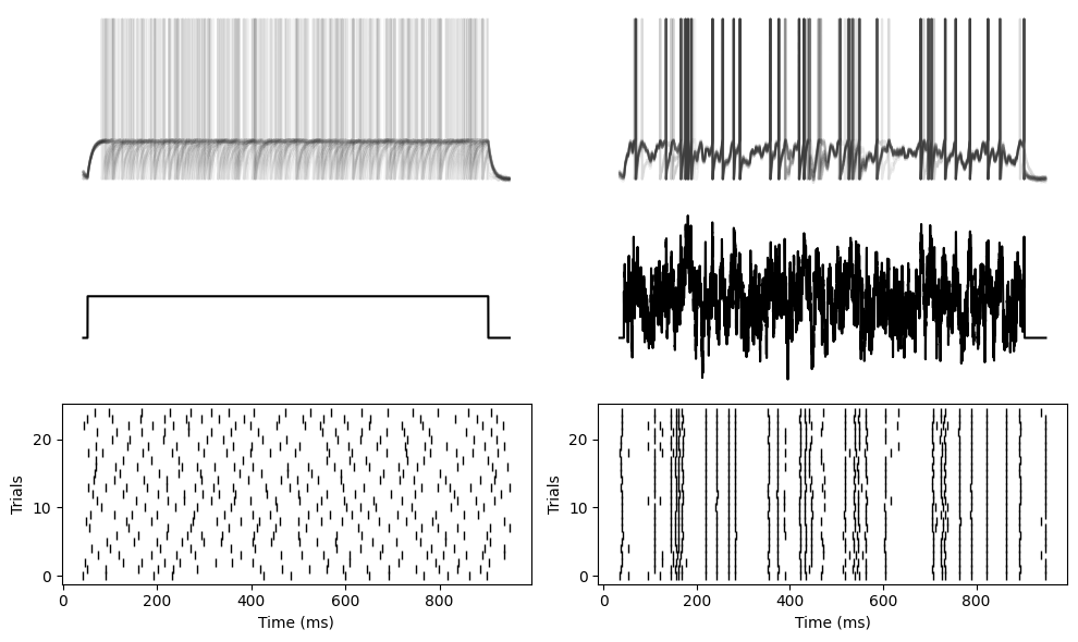
And same with a non-leaky integrate-and-fire neuron.
figure(figsize=(10, 6))

# Neuron equations and parameters
tau = 10*ms
sigma = .03
eqs_neurons = '''
dx/dt = (.15*I) / tau + sigma * (2 / tau)**.5 * xi : 1
I = I_shared*int((t>10*ms) and (t<950*ms)) : 1
I_shared : 1 (linked)
'''

start_scope()

# The common input
N = 25
neuron_input = NeuronGroup(1, 'x = 1.5 : 1', method='euler')

# The noisy neurons receiving the same input
neurons = NeuronGroup(N, model=eqs_neurons, threshold='x > 1',
                      reset='x = 0', refractory=5*ms, method='euler')
neurons.x = 'rand()*0.2'
neurons.I_shared = linked_var(neuron_input, 'x') # input.x is continuously fed into neurons.I
spikes = SpikeMonitor(neurons)
M = StateMonitor(neurons, ('x', 'I'), record=True)

run(1000*ms)

def add_spike_peak(x, t, i):
    T = array(rint(t/defaultclock.dt), dtype=int)
    y = x.copy()
    y[T, i] = 4
    return y

ax_top = subplot(321)
plot(M.t/ms, add_spike_peak(M.x[:].T, spikes.t[:], spikes.i[:]), '-k', alpha=0.05)
ax_top.set_frame_on(False)
xticks([])
yticks([])
ax_mid = subplot(323)
plot(M.t/ms, M.I[0], '-k')
ax_mid.set_frame_on(False)
xticks([])
yticks([])
subplot(325)
plot(spikes.t/ms, spikes.i, '|k')
xlabel('Time (ms)')
ylabel('Trials')

start_scope()

# The common noisy input
N = 25
tau_input = 3*ms
neuron_input = NeuronGroup(1, 'dx/dt = (1.5-x) / tau_input + (2 /tau_input)**.5 * xi : 1', method='euler')

# The noisy neurons receiving the same input
neurons = NeuronGroup(N, model=eqs_neurons, threshold='x > 1',
                      reset='x = 0', refractory=5*ms, method='euler')
neurons.x = 'rand()*0.2'
neurons.I_shared = linked_var(neuron_input, 'x') # input.x is continuously fed into neurons.I
spikes = SpikeMonitor(neurons)
M = StateMonitor(neurons, ('x', 'I'), record=True)

run(1000*ms)

ax = subplot(322, sharey=ax_top)
plot(M.t/ms, add_spike_peak(M.x[:].T, spikes.t[:], spikes.i[:]), '-k', alpha=0.05)
ax.set_frame_on(False)
xticks([])
yticks([])
ax = subplot(324, sharey=ax_mid)
plot(M.t/ms, M.I[0], '-k')
ax.set_frame_on(False)
xticks([])
yticks([])
subplot(326)
plot(spikes.t/ms, spikes.i, '|k')
xlabel('Time (ms)')
ylabel('Trials')

tight_layout()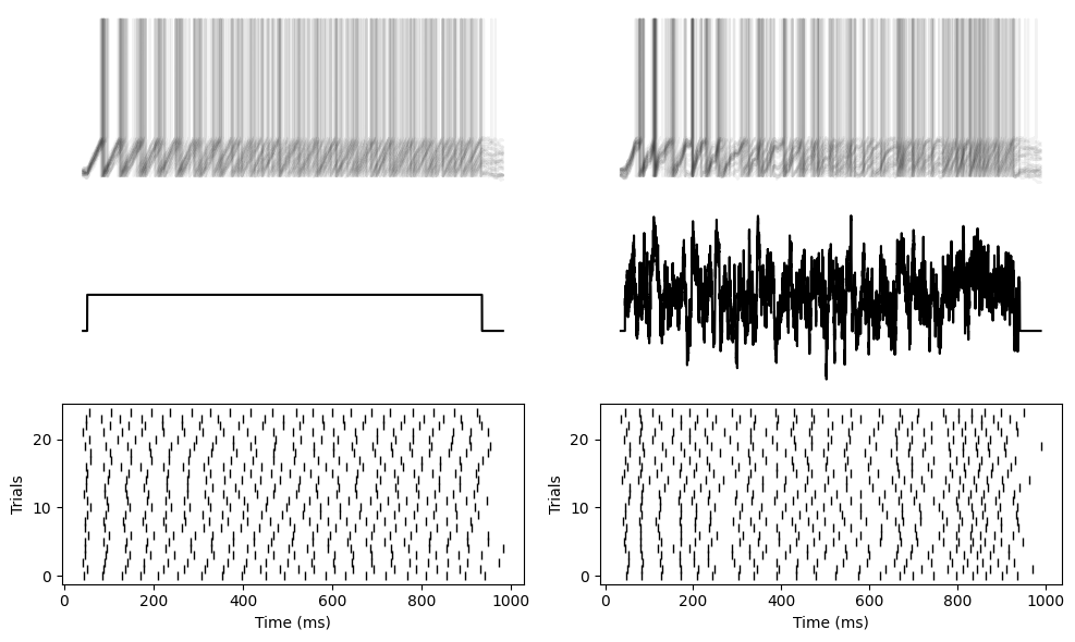
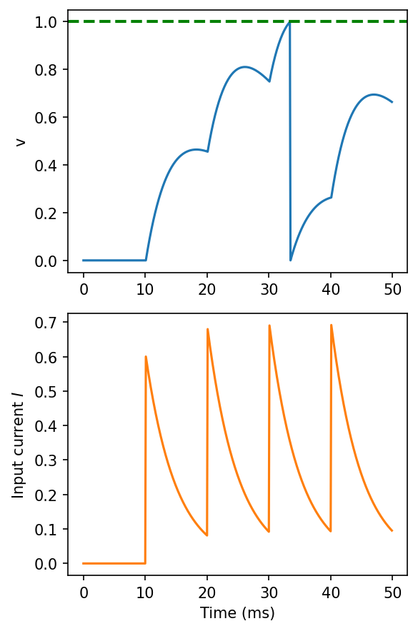
LIF with synapses
start_scope()

duration = 50*ms

eqs = '''
dv/dt = (4*I-v)/(15*ms) : 1
dI/dt = -I/(5*ms) : 1
'''
G_out = NeuronGroup(1, eqs, threshold='v>1', reset='v=0', method='euler')
nspikes_in = 100
timesep_in = 10*ms
G_in = SpikeGeneratorGroup(1, [0]*nspikes_in, (1+arange(nspikes_in))*timesep_in)
S = Synapses(G_in, G_out, on_pre='I += 0.6')
S.connect(p=1)
M = StateMonitor(G_out, ('v', 'I'), record=True)
run(duration)

figure(figsize=(4, 6), dpi=150)
subplot(211)
plot(M.t/ms, M.v[0], label='v')
axhline(1, ls='--', c='g', lw=2)
ylabel('v')
subplot(212)
plot(M.t/ms, M.I[0], label='I', c='C1')
xlabel('Time (ms)')
ylabel('Input current $I$')

tight_layout()
Adaptive threshold LIF neuron
start_scope()

duration = 150*ms

eqs = '''
dv/dt = -v/(15*ms) : 1
dvt/dt = (1-vt)/(50*ms) : 1
'''
G_out = NeuronGroup(2, eqs, threshold='v>vt', reset='v=0; vt+=0.4*i', method='euler')
G_out.vt = 1
nspikes_in = 100
timesep_in = 2*ms
G_in = SpikeGeneratorGroup(1, [0]*nspikes_in, (1+arange(nspikes_in))*timesep_in)
S = Synapses(G_in, G_out, on_pre='v += 0.3')
S.connect(p=1)
M = StateMonitor(G_out, ('v', 'vt'), record=True)
run(duration)
figure(figsize=(8, 4))
subplot(211)
plot(M.t/ms, M.v[0])
plot(M.t/ms, M.vt[0], ls='--', c='g', lw=2)
ylabel('v')
title('Standard LIF')
subplot(212)
plot(M.t/ms, M.v[1])
plot(M.t/ms, M.vt[1], ls='--', c='g', lw=2)
xlabel('Time (ms)')
ylabel('v')
title('Adaptive threshold')
tight_layout()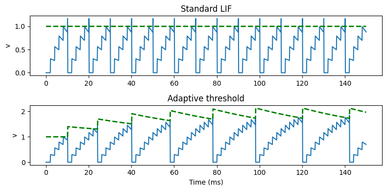
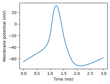
Hodgkin-Huxley neuron
start_scope()

duration = 3*ms

# Parameters
area = 20000*umetre**2
Cm = 1*ufarad*cm**-2 * area
gl = 5e-5*siemens*cm**-2 * area
El = -65*mV
EK = -90*mV
ENa = 50*mV
g_na = 100*msiemens*cm**-2 * area
g_kd = 30*msiemens*cm**-2 * area
VT = -63*mV

# The model
eqs = Equations('''
dv/dt = (gl*(El-v) - g_na*(m*m*m)*h*(v-ENa) - g_kd*(n*n*n*n)*(v-EK) + I)/Cm : volt
dm/dt = 0.32*(mV**-1)*4*mV/exprel((13.*mV-v+VT)/(4*mV))/ms*(1-m)-0.28*(mV**-1)*5*mV/exprel((v-VT-40.*mV)/(5*mV))/ms*m : 1
dn/dt = 0.032*(mV**-1)*5*mV/exprel((15.*mV-v+VT)/(5*mV))/ms*(1.-n)-.5*exp((10.*mV-v+VT)/(40.*mV))/ms*n : 1
dh/dt = 0.128*exp((17.*mV-v+VT)/(18.*mV))/ms*(1.-h)-4./(1+exp((40.*mV-v+VT)/(5.*mV)))/ms*h : 1
I = 0.7*nA * 8 : amp
''')
group = NeuronGroup(1, eqs, method='exponential_euler', dt=0.01*ms)
group.v = El

monitor = StateMonitor(group, 'v', record=True)

run(duration)

figure(figsize=(4,3))
plot(monitor.t/ms, monitor.v[0]/mV)
xlabel('Time (ms)')
_ = ylabel('Membrane potential (mV)')  # Suppress output