Reservoir computing
Let’s start with reservoir computing, also known as “liquid state machines” and “echo state networks” in different contexts.
In this setup we start with some time varying input sequence connected to a randomly recurrently connected group of neurons.
The connections included in the marked red section are not trained. The recurrent group is connected to a linear readout layer which is trained with a supervised algorithm to reproduce a desired time-varying output.
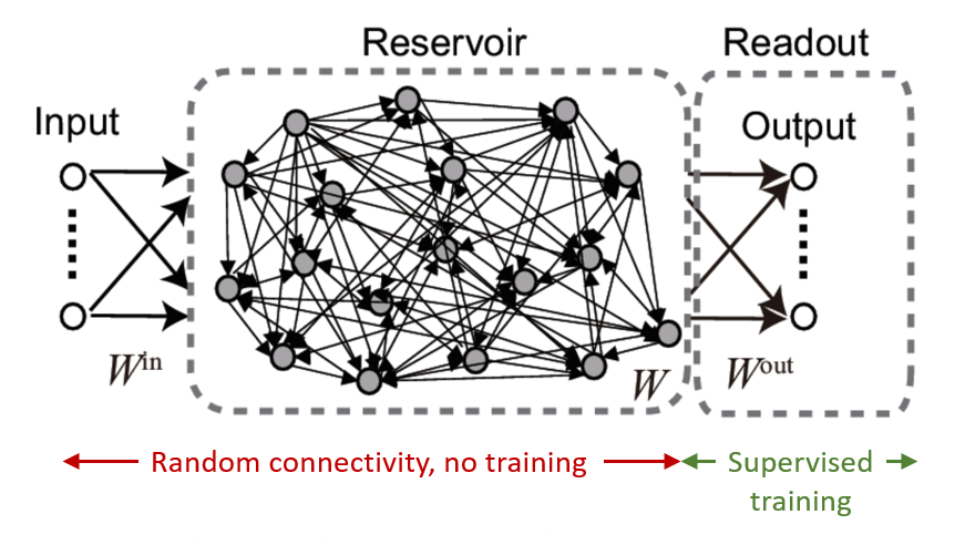
Figure 1:Reservoir computing setup.
You initialise the recurrent neurons with weights which put the network dynamics into a near chaotic state. The idea is that near chaos, you will find a rich set of trajectories in the dynamics of these neurons, and by doing a linear readout you can approximate any dynamics you like.
And this works!
You can prove that this setup allows you to approximate any time-varying function, with enough neurons. Here’s an example of a target trajectory and a reconstruction using reservoir computing.
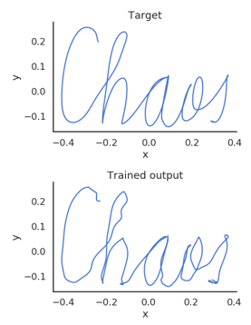
Figure 2:Example of a target trajectory and a reconstruction using reservoir computing.
There are lots of variants of this, for example with spiking neural networks you can add unsupervised training to the reservoir neurons using STDP.
A particularly interesting variant is FORCE training, where you write the recurrent weights as a sum of a fixed term that induces chaos, and a trainable term that can be trained with a recursive least squares algorithm.
For more
Evolutionary algorithms
Another approach is to use global optimisation algorithms that don’t require derivatives.
A particularly successful approach pioneered by Katie Schuman Schuman et al., 2020 is to use evolutionary algorithms. In these algorithms you generate a population of networks, evaluate them, and then create new networks by mixing up the most successful networks, repeating until you get good performance.
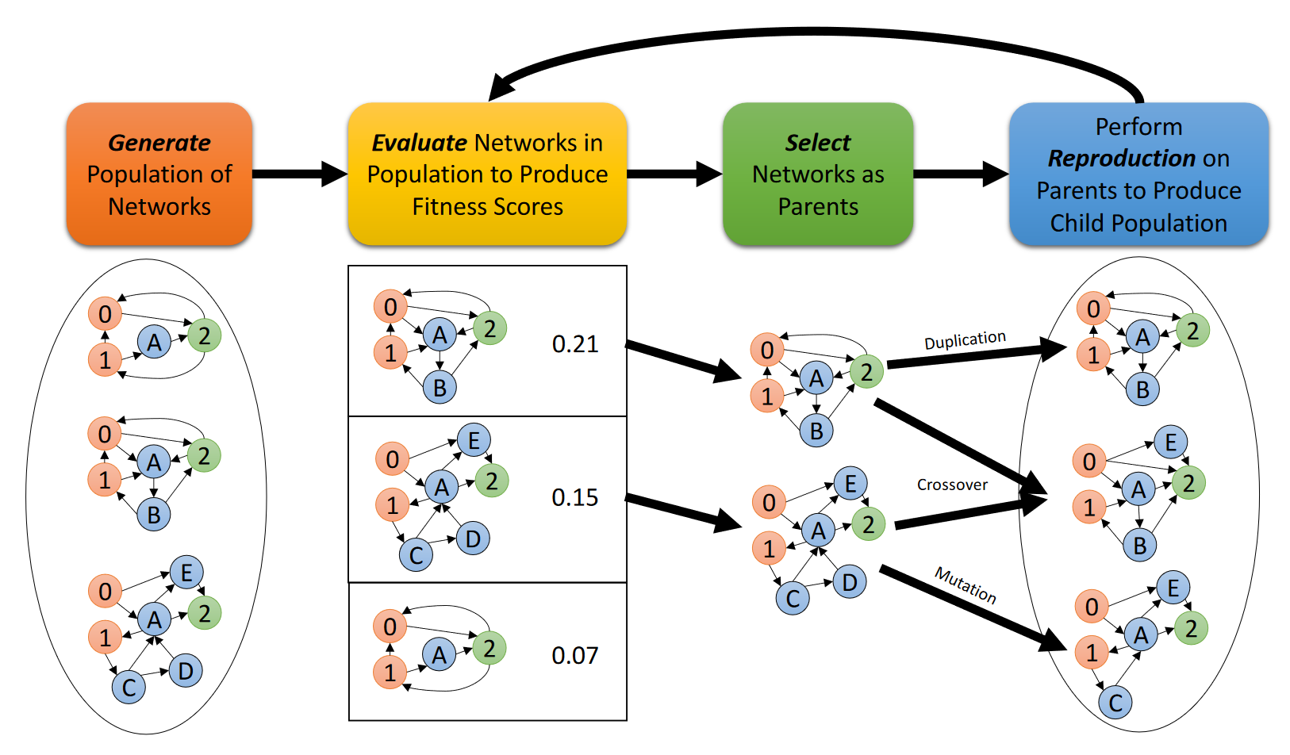
Figure 3:Training SNNs with evolutionary algorithms Schuman et al., 2020.
Here’s an example network evolved with this method to classify breast cancer images.
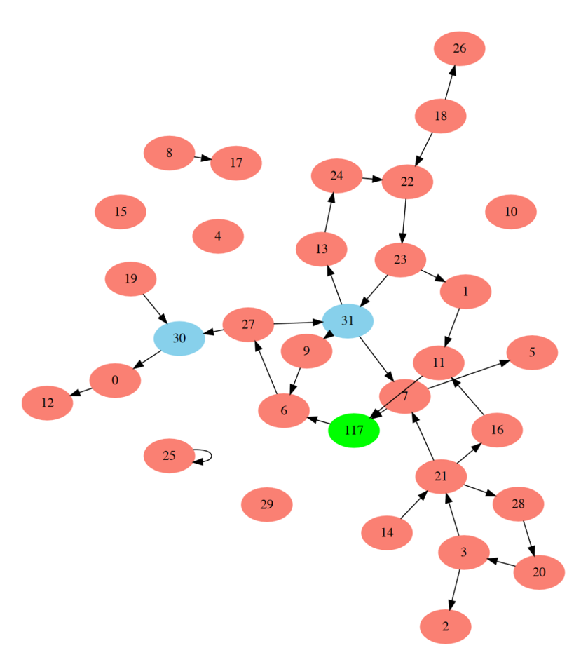
Figure 4:Example network evolved to classify breast cancer images Schuman et al., 2020.
The advantage of this method is that it can find surprising architectures like this one that you might never otherwise have found. But, it does tend to be computationally demanding and limited to fairly small networks like this.
It’s also been used to train neuromorphic hardware that we’ll talk about later in this course, for example a controller for this little robot.
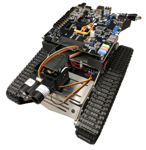
Figure 5:Robot controlled by neuromorphic hardware Mitchell et al., 2017.
You can see an example of the sort of network it finds. Another advantage here is that you can easily adapt it to the type of hardware available. In this case, a field programmable gate array or FPGA.
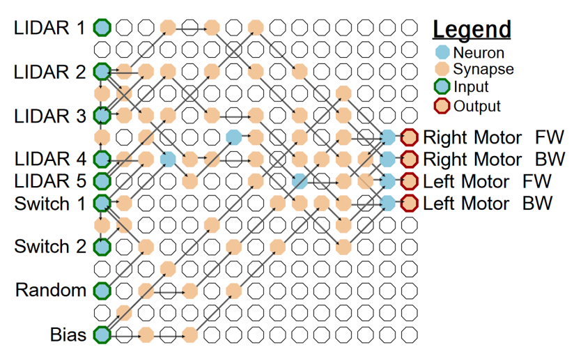
Figure 6:Robot controller network Mitchell et al., 2017.
And here’s an example of a trajectory showing that this robot was able to learn to drive around, avoid obstacles, etc.
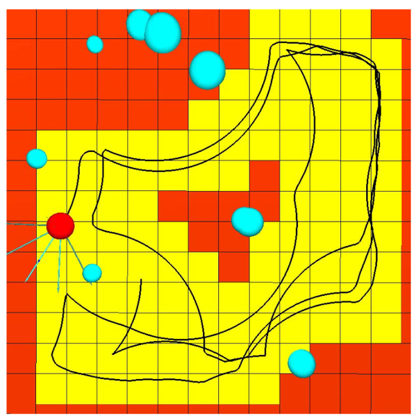
Figure 7:Robot trajectory Mitchell et al., 2017.
Converting artificial to spiking neural networks
Rather than trying to work with spiking neural networks directly, we can start by doing something we know how to do, like training an artificial neural network, and then convert the result into a spiking neural network.
There’s a huge literature on this but I’m just going to mention two approaches from Hunsberger & Eliasmith (2015).
Soft-LIF
The first starts by creating a non-spiking artificial neuron called a soft-LIF that approximates the input-output behavior of a spiking neuron.
You then train this soft-LIF network with standard algorithms, possibly adding training noise to make it more noise robust.
Then just replace those soft-LIF neurons with real LIF neurons and it works fairly well.
Eliasmith and colleagues later took this sort of approach much further, creating a very general method called the Neural Engineering Framework (NEF).
Neural engineering framework
In this approach, you can directly implement vector function and differentials by encoding input values into a random high dimensional overcomplete representation
And then linearly decoding this, which they show allows you to approximate almost any function.
They implemented this in a comprehensive software package Nengo so it’s easy to try it out if you’re interested.
Once you have these building blocks, it’s easy to then convert an ANN that is composed of these building blocks into their framework and implement it with spiking neurons.
Restricting to a single spike
The last method we’ll look at in this section is making the network differentiable by limiting each neuron to only be able to fire a single spike.
This might seem like a crazy limitation, but there’s actually a good reason to try this coming from Simon Thorpe and colleagues.
They noted that primate brains are able to classify and respond to quite complicated visual stimuli, like distinguishing between food and not-food, with as little as a 100ms delay.
From studying the anatomy, they knew that to go from the visual system to the motor system that registered the response, the signal would have to go through around 10 layers.
Since cortical neurons usually fire only at most around 100 spikes per sec, that means that in the 10ms that each layer has to process, it likely only fires 0 or 1 spikes.
So it must be possible to do quite complex tasks with each neuron firing only 0 or 1 spikes. Kheradpisheh & Masquelier (2020) implemented this idea.
They set up a network of integrate and fire neurons (note: not leaky integrate and fire), and only allowed them to fire one spike per stimulus presented.
With that limitation in place, they could write the output spike time of a neuron analytically in terms of the input spike times and weights. This function is differentiable, so we can apply backprop to train these networks.
They found that this gave excellent performance at the same types of visual classification tasks that Simon Thorpe had earlier studied in primates. For example, they could very reliably distinguish between faces and motorcycles in this dataset.
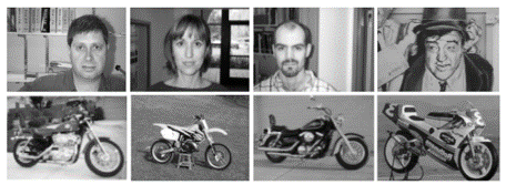
Figure 8:Distinguishing between faces and motorcycles visual classification task Kheradpisheh & Masquelier, 2020.
OK, that’s enough for these limited gradient approaches. As usual, this section has only scratched the surface, and it’s still a very active area of research.
- Nicola, W., & Clopath, C. (2017). Supervised learning in spiking neural networks with FORCE training. Nature Communications, 8(1). 10.1038/s41467-017-01827-3
- Schuman, C. D., Mitchell, J. P., Patton, R. M., Potok, T. E., & Plank, J. S. (2020). Evolutionary Optimization for Neuromorphic Systems. Proceedings of the Neuro-Inspired Computational Elements Workshop, 1–9. 10.1145/3381755.3381758
- Mitchell, J. P., Bruer, G., Dean, M. E., Plank, J. S., Rose, G. S., & Schuman, C. D. (2017). NeoN: Neuromorphic control for autonomous robotic navigation. 2017 IEEE International Symposium on Robotics and Intelligent Sensors (IRIS), 136–142. 10.1109/iris.2017.8250111
- Hunsberger, E., & Eliasmith, C. (2015). Spiking Deep Networks with LIF Neurons. arXiv. 10.48550/ARXIV.1510.08829
- Kheradpisheh, S. R., & Masquelier, T. (2020). Temporal Backpropagation for Spiking Neural Networks with One Spike per Neuron. International Journal of Neural Systems, 30(06), 2050027. 10.1142/s0129065720500276