Introduction
We’re now going to explain how to train spiking neural networks with the surrogate gradient method. This method isn’t perfect, and we’ll talk about some of its drawbacks later, but at the moment it seems to be a very good balance of flexibility and efficiency. There’s a lot of research going on in this area at the moment, and there will likely be big advances in the next few years.
Unrolling recurrent neural networks
The surrogate gradient method treats a spiking neural network as a very particular sort of recurrent neural network. That’s true even if the spiking neural network doesn’t have recurrent connections, because the fact that the internal state of a neuron at one time step depends on its internal state at a previous time step makes it implicitly recurrent. With that in mind, let’s quickly look at how you can train a recurrent neural network.
First, we define the network like this. We have parameters θ that could be weights, biases, etc. We have a time varying input fed into a recurrent network whose internal state is . That gets fed into an output layer , which has an associated loss function .
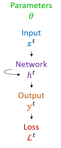
Figure 1:Recurrent neural network definition.
Now we unroll this through time to see the dependencies more clearly. You can see that the network state at time for example is affected by the inputs at time but also the network state at time , and so on.
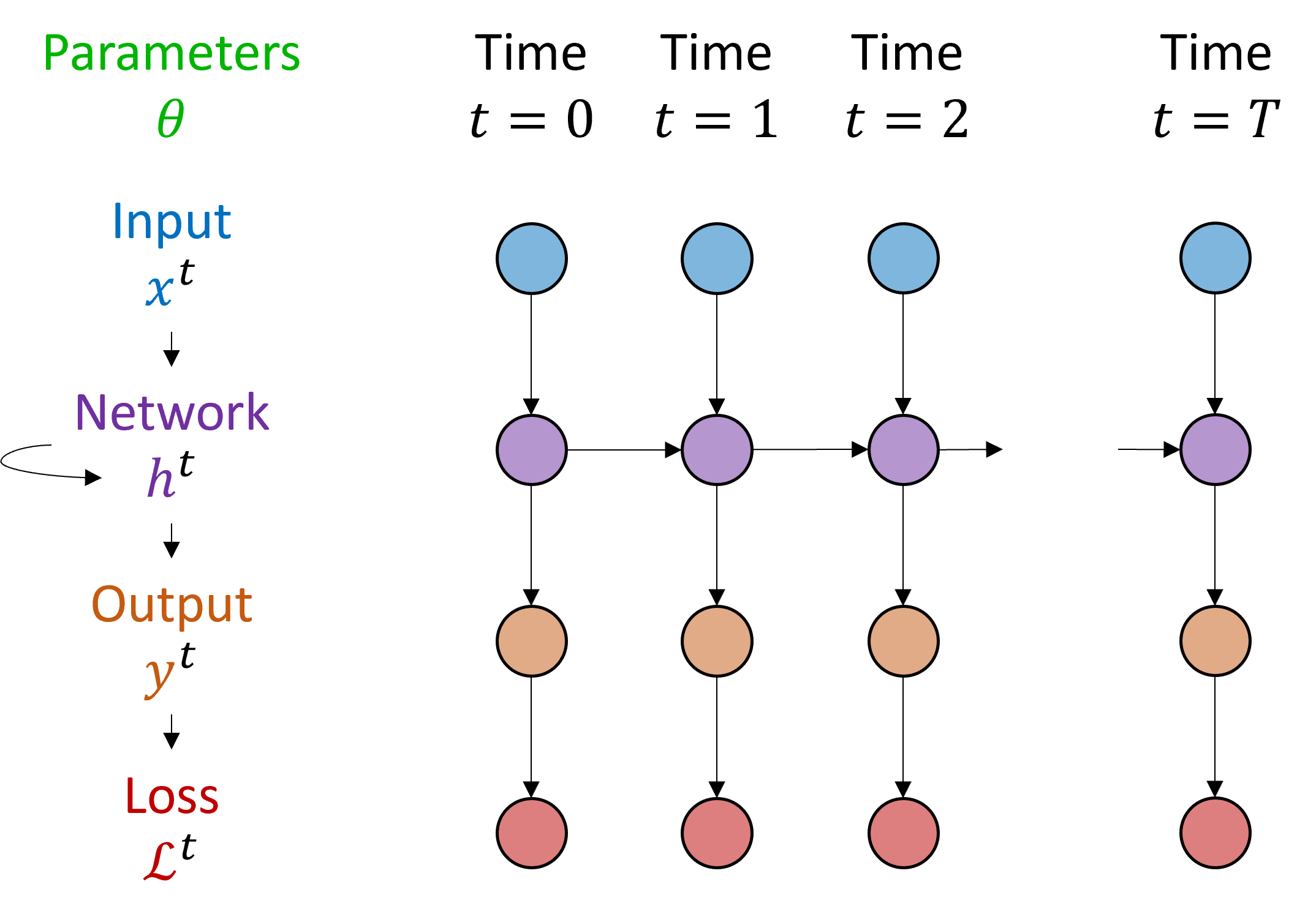
Figure 2:Unrolled recurrent neural network.
We can write a mathematical definition of the network as follows:
Here is the function that takes the network state, input and parameters, and returns the updated network state. This function could be the application of a single layer or it could be the result of applying multiple layers, or anything else really.
We can expand this function out to get a feel for what happens. In the first time step, you just get the definition above. For the second time step, we can expand out the to get the result only in terms of θ, the initial state and the inputs. And we can continue like that for all the time steps. In the final time step we apply another function .
And then we have an expression for the loss only in terms of the parameters theta and the inputs.
That means we can compute a gradient of the loss with respect to the parameters using the chain rule. And with that, we can write a gradient descent update rule, as we’ve seen before. The gradient can be computed with the chain rule, and the update rule is:
That all looks complicated but actually modern machine learning toolboxes do all the work for us with their autodifferentiation packages. We just write the forward pass and it handles efficiently computing the gradients using the chain rule, applying the update rule, etc. This algorithm is called backpropagation through time (BPTT), because it’s the standard backpropagation algorithm applied to a function that is repeatedly applied through time.
Spiking neuron: the surrogate gradient
Now let’s take this idea and apply it to a spiking neural network. This section follows on from Why we can’t do it so go ahead and re-read that before continuing.
The key point here is that we can write equations to update the internal network state from one time step to the next like the function seen previously. This is entirely composed of nicely differentiable functions with one exception, the Heaviside function which is used in computing whether or not a neuron has crossed a threshold and fired a spike.
This function is discontinuous and has a derivative that is zero everywhere except at , which means when we compute gradients using the chain rule or an autodifferentiation package, we’ll just get zeros and no updates will happen.
The solution, which is a little strange, is to keep the function as it is in the forward pass, but whenever we see a copy of the derivative of , we replace it with the derivative of a smoothed version of the Heaviside function.

The intuition here is that if we have a loss landscape with discontinuous jumps corresponding to when a change in gradients causes there to be one more or fewer spikes, then smoothing the Heaviside function will smooth out those jumps in the loss landscape.
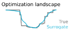
An example function we can use is the logistic sigmoid function, which has a nice simple derivative.
But it turns out that the choice of smoothing function doesn’t actually matter that much, the algorithm is very robust to a wide range of functions Zenke & Vogels, 2021.
That all sounds nice in theory, but we have these lovely autodifferentiation functions and implementing this idea looks like it’ll be a nightmare.
Implementation with PyTorch
Actually, it’s not as bad as it seems. PyTorch and other libraries allow you to overwrite the default implementation of the gradient computation. I don’t think this was designed for implementing surrogate gradients, but it does the job nicely. Let’s look at the code.
# Derive from PyTorch to make the magic happen
class SurrogateHeaviside(torch.autograd.Function):
    # In the forward pass, just return Heaviside
    @staticmethod
    def forward(ctx, input):
        ctx.save_for_backward(input)
        return torch.heaviside(input, 0)
    # In the backward pass, return derivative of sigmoid
    @staticmethod
    def backward(ctx, grad_output):
        input, = ctx.saved_tensors
        beta = 5
        s = torch.sigmoid(beta*input)
        grad = grad_output*beta*s*(1-s)
        return grad
# Now use this instead of Heaviside
surrogate_heaviside  = SurrogateHeaviside.apply
We start by defining a class SurrogateHeaviside. This derives from the PyTorch autograd.Function class to make it compatible with PyTorch. We’ll use this to create a new magic surrogate version of the Heaviside function that will do exactly what we want.
PyTorch requires you to implement two methods. The first is what happens for the forward pass. We just want it to return the standard Heaviside function, and for our purposes this context save for backward is just boilerplate to make it play nicely with PyTorch.
The second method is the backward pass. It starts in the same way with some boilerplate that lets us get the input and the gradient of the output (because we’re going backwards).
Then we compute our new derivative. We set a parameter beta which specifies how steep the sigmoid function is, and then compute the derivative using the previous formula. Note that we multiply the derivative by the output gradient which was given us by PyTorch.
And that’s it. We instantiate this class and just use that instead of the Heaviside function. And now, by magic, our spiking neural network can be used with autodifferentiation and we can use any optimisation algorithm, like stochastic gradient descent, the Adam learning rule, etc.
It works!
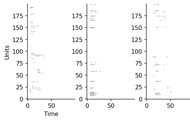
Here’s an example using the spiking Heidelberg digits (SHD) dataset. This is a database constructed by having several different speakers read the digits 0 through 9 in English and German, taking those sound waves and feeding them into a fairly detailed model of how the early auditory system processes sounds to produce spike raster plots like these. On each figure, the y axis is the neuron index, with the bottom rows corresponding to low sound frequencies, and the upper rows high frequencies. The x-axis is time. If you’ve seen spectrograms of sound before, this should look somewhat familiar because at a very rough level, that’s what the early part of the auditory system is doing.

Figure 5:Spike raster plots from the Spiking Heidelberg Digits dataset.
We can train a spiking neural network model to take these as input and ask it to classify the digit, and it’s able to do the task. Here are some of the intermediate spike trains from model neurons after training.
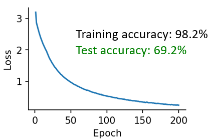
You can see that with training the loss curve has a familiar shape, and at the end we get a test accuracy of about 70% which isn’t too bad for a classification task with a chance accuracy of 5% and only 200 spiking neurons.
Friedemann Zenke, who built this dataset, keeps a table of the best performers, and at the time of recording the best was around 95%. The key innovation there was to allow for trainable delays between neurons. That’s great performance, but I’m pretty sure it’ll go higher. Maybe one of you can beat that score?
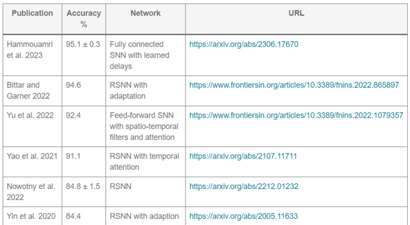
Figure 8:Friedemann Zenke’s table of best performers on the SHD dataset (as of 2024/10/31).
Before we get too excited, there are some issues with this method.
Issues
Resource hungry
The first is that despite making it feasible to train spiking neural networks at complex tasks, it is still quite resource hungry.
To get a feeling for this, let’s say we have neurons, fully connected to each other, and we run the network for time steps.
The algorithm will use computation time per simulation time step.
It will also take storage space. This is the real killer because if you want to run these algorithms fast, you want to run them on a GPU, and this means you are very limited in terms of how much RAM you have available. You’re essentially making a copy of the complete network state for every time step of the simulation, which racks up fast. For a time step of 1 millisecond, you’re making 1000 copies of the network state per second of simulated time.
Hard to initialise well
Another issue is that it’s hard to initialise these networks well. You want an initial state with a couple of key properties:
It should produce a reasonable number of spikes at every layer: not too much and not too little or it will be hard to find a good solution.
You want the network to be initialised in a state where gradients neither vanish nor explode, a common problem with training deep or recurrent neural networks.
Various ideas have been proposed for this, including but not limited to:
- Initialising in a brain-like state Rossbroich et al., 2022.
- Analytically computing the variances in both the forward and backwards pass Perez-Nieves & Goodman, 2023. Note that the maths for this gets very hairy, very fast, and is highly specific to the type of neurons you’re using, which means this analytical solution is harder to deploy in practice than we might like.
Uses non-local information
A final issue we wanted to mention is that like any backprop through time algorithm, it uses non-local information that wouldn’t be available to real neurons in the brain, meaning that without some additional work it’s not a good candidate for how the brain itself does learning. That doesn’t mean it’s not a good way to train spiking neural networks in the abstract, however, and doesn’t stop us from using it to model what the brain is doing in other ways.
Application: neural heterogeneity
On that note, we’d like to finish with a bit of self advertising, by talking about a study done by one of the team’s PhD students using surrogate gradient descent to tell us something about how the brain might work Perez-Nieves et al., 2021.
The idea was to start from the standard leaky integrate-and-fire neuron equations, but instead of just training the synaptic weights, we also make the time constants τ trainable too. In terms of implementation in PyTorch, that’s almost as simple as a single line modification of the code, although there is some work to do to stop the algorithm getting stuck or running into numerical integration issues.
The results from this were really neat:
We get a big improvement in performance, especially for temporally complex datasets like the Heidelberg digits dataset we saw before. We get this for a tiny increase in the number of parameters, because we’ve only added one new trainable parameter per neuron, which is , and not increased the number of synaptic weights, of which there are .
The method was more robust when tested out of the distribution of the training set.
The time constants we learned matched what we see in experimentally recorded brain data. Specifically, regardless of how we initialised the time constants, for each dataset they always found their way to a characteristic distribution that is roughly log normal or Gamma distributed. This is exactly what you see in the brain across multiple different regions and animal types, including humans.
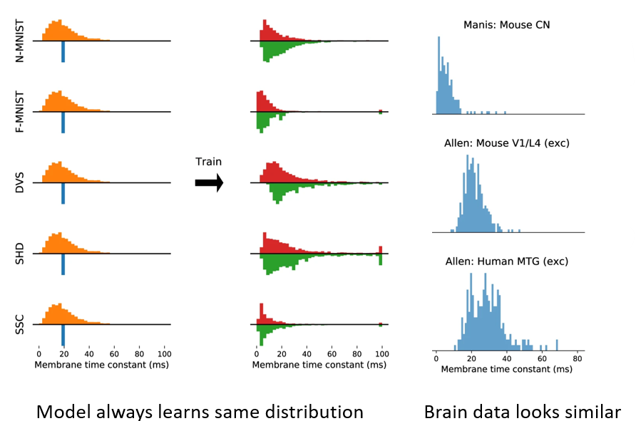
It’s not conclusive, but we think this suggests that having neurons that aren’t all the same can allow the brain to do much more without a big increase in required resources.
Incidentally, these experimentally recorded distributions were obtained from the Allen Institute database, which is openly and freely available to explore with a nice Python API, so you should have a play around with that.
Next steps
OK, that’s all for this section on surrogate gradient descent. We strongly advise you to spend some time getting to grips with it more detail, starting from Friedemann Zenke’s excellent SPyTorch tutorial which builds up the code to run this step by step from scratch until you have a network that can solve the Spiking Heidelberg digits data set.
This week’s exercise starts by going through the first part of this tutorial and then applying it to a different problem. We’ve also included some reading material if you want to get a bit deeper into the maths of surrogate gradient descent, although do be warned you might need to set aside a few days to go through this.
- Zenke, F., & Vogels, T. P. (2021). The Remarkable Robustness of Surrogate Gradient Learning for Instilling Complex Function in Spiking Neural Networks. Neural Computation, 33(4), 899–925. 10.1162/neco_a_01367
- Rossbroich, J., Gygax, J., & Zenke, F. (2022). Fluctuation-driven initialization for spiking neural network training. Neuromorphic Computing and Engineering, 2(4), 044016. 10.1088/2634-4386/ac97bb
- Perez-Nieves, N., & Goodman, D. F. M. (2023). Spiking Network Initialisation and Firing Rate Collapse. arXiv. 10.48550/ARXIV.2305.08879
- Perez-Nieves, N., Leung, V. C. H., Dragotti, P. L., & Goodman, D. F. M. (2021). Neural heterogeneity promotes robust learning. Nature Communications, 12(1). 10.1038/s41467-021-26022-3